
20 Covariance
Another of the uses of the F distribution is testing two variances. It is often desirable to compare two variances rather than two averages. For instance, college administrators would like two college professors grading exams to have the same variation in their grading. In order for a lid to fit a container, the variation in the lid and the container should be the same. A supermarket might be interested in the variability of check-out times for two checkers.
In order to perform a F test of two variances, it is important that the following are true:
Unlike most other tests in this book, the F test for equality of two variances is very sensitive to deviations from normality. If the two distributions are not normal, the test can give higher p-values than it should, or lower ones, in ways that are unpredictable. Many texts suggest that students not use this test at all, but in the interest of completeness we include it here.
Suppose we sample randomly from two independent normal populations. Let  and
and  be the population variances and
  and
and  be the sample variances. Let the
sample sizes be n1 and n2. Since we are interested in comparing the two sample variances, we use the F ratio:
![F=\frac{\left[\frac{{\left({s}_{1}\right)}^{2}}{{\left({\sigma }_{1}\right)}^{2}}\right]}{\left[\frac{{\left({s}_{2}\right)}^{2}}{{\left({\sigma }_{2}\right)}^{2}}\right]}](https://uhlibraries.pressbooks.pub/app/uploads/quicklatex/quicklatex.com-f327c17f5258ba27b15b086541d6a88c_l3.png "Rendered by QuickLaTeX.com")
F has the distribution F ~ F(n1 – 1, n2 – 1)
where n1 – 1 are the degrees of freedom for the numerator and n2 – 1 are the degrees of freedom for the denominator.
If the null hypothesis is  , then the F Ratio becomes
 ![F=\frac{\left[\frac{{\left({s}_{1}\right)}^{2}}{{\left({\sigma }_{1}\right)}^{2}}\right]}{\left[\frac{{\left({s}_{2}\right)}^{2}}{{\left({\sigma }_{2}\right)}^{2}}\right]}=\frac{{\left({s}_{1}\right)}^{2}}{{\left({s}_{2}\right)}^{2}}](https://uhlibraries.pressbooks.pub/app/uploads/quicklatex/quicklatex.com-0c88a685ed563257c84e43a615355565_l3.png "Rendered by QuickLaTeX.com") .
.
The F ratio could also be  .
.
It depends on Ha and on which sample variance is larger.
If the two populations have equal variances, then and are close in value and  is close to one. But if the two population variances are very different, and tend to be very different, too. Choosing as the larger sample variance causes the ratio
  to be greater than one. If and are far apart, then is a large number.
Therefore, if F is close to one, the evidence favors the null hypothesis (the two population variances are equal). But if F is much larger than one, then the evidence is against the null hypothesis. A test of two variances may be left, right, or two-tailed.
Two college instructors are interested in whether or not there is any variation in the way they grade math exams. They each grade the same set of 30 exams. The first instructor’s grades have a variance of 52.3. The second instructor’s grades have a variance of 89.9. Test the claim that the first instructor’s variance is smaller. (In most colleges, it is desirable for the variances of exam grades to be nearly the same among instructors.) The level of significance is 10%.
Let 1 and 2 be the subscripts that indicate the first and second instructor, respectively.
n1 = n2 = 30.
H0: and Ha: 
Calculate the test statistic: By the null hypothesis  , the F statistic is:
![F=\frac{\left[\frac{{\left({s}_{1}\right)}^{2}}{{\left({\sigma }_{1}\right)}^{2}}\right]}{\left[\frac{{\left({s}_{2}\right)}^{2}}{{\left({\sigma }_{2}\right)}^{2}}\right]}=\frac{{\left({s}_{1}\right)}^{2}}{{\left({s}_{2}\right)}^{2}}=\frac{52.3}{89.9}=0.5818](https://uhlibraries.pressbooks.pub/app/uploads/quicklatex/quicklatex.com-d867bb4db69cb77b29b88e661a0a7b51_l3.png "Rendered by QuickLaTeX.com")
Distribution for the test:F29,29 where n1 – 1 = 29 and n2 – 1 = 29.
Graph: This test is left tailed.
Draw the graph labeling and shading appropriately.
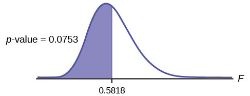
Probability statement:p-value = P(F < 0.5818) = 0.0753
Compare α and the p-value:α = 0.10 α > p-value.
Make a decision: Since α > p-value, reject H0.
Conclusion: With a 10% level of significance, from the data, there is sufficient evidence to conclude that the variance in grades for the first instructor is smaller.
Press STAT and arrow over to TESTS. Arrow down to D:2-SampFTest. Press ENTER. Arrow to Stats and press ENTER. For Sx1, n1, Sx2, and n2, enter 
30, 
30. Press ENTER after each. Arrow to σ1: and  σ2
σ2ENTER. Arrow down to Calculate and press ENTER. F = 0.5818 and p-value = 0.0753. Do the procedure again and try Draw instead of Calculate.
The New York Choral Society divides male singers up into four categories from highest voices to lowest: Tenor1, Tenor2, Bass1, Bass2. In the table are heights of the men in the Tenor1 and Bass2 groups. One suspects that taller men will have lower voices, and that the variance of height may go up with the lower voices as well. Do we have good evidence that the variance of the heights of singers in each of these two groups (Tenor1 and Bass2) are different?
| Tenor1 | Bass2 | Tenor 1 | Bass 2 | Tenor 1 | Bass 2 |
|---|---|---|---|---|---|
| 69 | 72 | 67 | 72 | 68 | 67 |
| 72 | 75 | 70 | 74 | 67 | 70 |
| 71 | 67 | 65 | 70 | 64 | 70 |
| 66 | 75 | 72 | 66 | 69 | |
| 76 | 74 | 70 | 68 | 72 | |
| 74 | 72 | 68 | 75 | 71 | |
| 71 | 72 | 64 | 68 | 74 | |
| 66 | 74 | 73 | 70 | 75 | |
| 68 | 72 | 66 | 72 |
The histograms are not as normal as one might like. Plot them to verify. However, we proceed with the test in any case.
Subscripts: T1= tenor1 and B2 = bass 2
The standard deviations of the samples are sT1 = 3.3302 and sB2 = 2.7208.
The hypotheses are
 and
and  (two tailed test)
The F statistic is 1.4894 with 20 and 25 degrees of freedom.
The p-value is 0.3430. If we assume alpha is 0.05, then we cannot reject the null hypothesis.
We have no good evidence from the data that the heights of Tenor1 and Bass2 singers have different variances (despite there being a significant difference in mean heights of about 2.5 inches.)
References
“MLB Vs. Division Standings – 2012.” Available online at http://espn.go.com/mlb/standings/_/year/2012/type/vs-division/order/true.
Chapter Review
The F test for the equality of two variances rests heavily on the assumption of normal distributions. The test is unreliable if this assumption is not met. If both distributions are normal, then the ratio of the two sample variances is distributed as an F statistic, with numerator and denominator degrees of freedom that are one less than the samples sizes of the corresponding two groups. A test of two variances hypothesis test determines if two variances are the same. The distribution for the hypothesis test is the F distribution with two different degrees of freedom.
- The populations from which the two samples are drawn are normally distributed.
- The two populations are independent of each other.
Formula Review
F has the distribution F ~ F(n1 – 1, n2 – 1)
F = 
If σ1 = σ2, then F = 
Use the following information to answer the next two exercises. There are two assumptions that must be true in order to perform an F test of two variances.
Name one assumption that must be true.
The populations from which the two samples are drawn are normally distributed.
What is the other assumption that must be true?
Use the following information to answer the next five exercises. Two coworkers commute from the same building. They are interested in whether or not there is any variation in the time it takes them to drive to work. They each record their times for 20 commutes. The first worker’s times have a variance of 12.1. The second worker’s times have a variance of 16.9. The first worker thinks that he is more consistent with his commute times and that his commute time is shorter. Test the claim at the 10% level.
State the null and alternative hypotheses.
H0: σ1 = σ2
Ha: σ1 < σ2
or
H0: 
Ha: 
What is s1 in this problem?
What is s2 in this problem?
4.11
What is n?
What is the F statistic?
0.7159
What is the p-value?
Is the claim accurate?
No, at the 10% level of significance, we do not reject the null hypothesis and state that the data do not show that the variation in drive times for the first worker is less than the variation in drive times for the second worker.
Use the following information to answer the next four exercises. Two students are interested in whether or not there is variation in their test scores for math class. There are 15 total math tests they have taken so far. The first student’s grades have a standard deviation of 38.1. The second student’s grades have a standard deviation of 22.5. The second student thinks his scores are lower.
State the null and alternative hypotheses.
What is the F Statistic?
2.8674
What is the p-value?
At the 5% significance level, do we reject the null hypothesis?
Reject the null hypothesis. There is enough evidence to say that the variance of the grades for the first student is higher than the variance in the grades for the second student.
Use the following information to answer the next three exercises. Two cyclists are comparing the variances of their overall paces going uphill. Each cyclist records his or her speeds going up 35 hills. The first cyclist has a variance of 23.8 and the second cyclist has a variance of 32.1. The cyclists want to see if their variances are the same or different.
State the null and alternative hypotheses.
What is the F Statistic?
0.7414
At the 5% significance level, what can we say about the cyclists’ variances?
Homework
Three students, Linda, Tuan, and Javier, are given five laboratory rats each for a nutritional experiment. Each rat’s weight is recorded in grams. Linda feeds her rats Formula A, Tuan feeds his rats Formula B, and Javier feeds his rats Formula C. At the end of a specified time period, each rat is weighed again and the net gain in grams is recorded.
| Linda’s rats | Tuan’s rats | Javier’s rats |
|---|---|---|
| 43.5 | 47.0 | 51.2 |
| 39.4 | 40.5 | 40.9 |
| 41.3 | 38.9 | 37.9 |
| 46.0 | 46.3 | 45.0 |
| 38.2 | 44.2 | 48.6 |
Determine whether or not the variance in weight gain is statistically the same among Javier’s and Linda’s rats. Test at a significance level of 10%.


- df(num) = 4; df(denom) = 4
- F4, 4
- 3.00
- 2(0.1563) = 0.3126. Using the TI-83+/84+ function 2-SampFtest, you get the test statistic as 2.9986 and p-value directly as 0.3127. If you input the lists in a different order, you get a test statistic of 0.3335 but the p-value is the same because this is a two-tailed test.
- Check student’t solution.
- Decision: Do not reject the null hypothesis; Conclusion: There is insufficient evidence to conclude that the variances are different.
A grassroots group opposed to a proposed increase in the gas tax claimed that the increase would hurt working-class people the most, since they commute the farthest to work. Suppose that the group randomly surveyed 24 individuals and asked them their daily one-way commuting mileage. The results are as follows.
| working-class | professional (middle incomes) | professional (wealthy) |
|---|---|---|
| 17.8 | 16.5 | 8.5 |
| 26.7 | 17.4 | 6.3 |
| 49.4 | 22.0 | 4.6 |
| 9.4 | 7.4 | 12.6 |
| 65.4 | 9.4 | 11.0 |
| 47.1 | 2.1 | 28.6 |
| 19.5 | 6.4 | 15.4 |
| 51.2 | 13.9 | 9.3 |
Determine whether or not the variance in mileage driven is statistically the same among the working class and professional (middle income) groups. Use a 5% significance level.
Refer to the data from [link].
Examine practice laps 3 and 4. Determine whether or not the variance in lap time is statistically the same for those practice laps.
Use the following information to answer the next two exercises. The following table lists the number of pages in four different types of magazines.
| home decorating | news | health | computer |
|---|---|---|---|
| 172 | 87 | 82 | 104 |
| 286 | 94 | 153 | 136 |
| 163 | 123 | 87 | 98 |
| 205 | 106 | 103 | 207 |
| 197 | 101 | 96 | 146 |
- H0: =
- Ha: ≠
- df(n) = 19, df(d) = 19
- F19,19
- 1.13
- 0.786
- Check student’s solution.
-
- Alpha:0.05
- Decision: Do not reject the null hypothesis.
- Reason for decision: p-value > alpha
- Conclusion: There is not sufficient evidence to conclude that the variances are different.
Which two magazine types do you think have the same variance in length?
Which two magazine types do you think have different variances in length?
The answers may vary. Sample answer: Home decorating magazines and news magazines have different variances.
Is the variance for the amount of money, in dollars, that shoppers spend on Saturdays at the mall the same as the variance for the amount of money that shoppers spend on Sundays at the mall? Suppose that the [link] shows the results of a study.
| Saturday | Sunday | Saturday | Sunday |
|---|---|---|---|
| 75 | 44 | 62 | 137 |
| 18 | 58 | 0 | 82 |
| 150 | 61 | 124 | 39 |
| 94 | 19 | 50 | 127 |
| 62 | 99 | 31 | 141 |
| 73 | 60 | 118 | 73 |
| 89 |
Are the variances for incomes on the East Coast and the West Coast the same? Suppose that [link] shows the results of a study. Income is shown in thousands of dollars. Assume that both distributions are normal. Use a level of significance of 0.05.
| East | West |
|---|---|
| 38 | 71 |
| 47 | 126 |
| 30 | 42 |
| 82 | 51 |
| 75 | 44 |
| 52 | 90 |
| 115 | 88 |
| 67 |
- H0: = =
- Ha: ≠
- df(n) = 7, df(d) = 6
- F7,6
- 0.8117
- 0.7825
- Check student’s solution.
-
- Alpha: 0.05
- Decision: Do not reject the null hypothesis.
- Reason for decision: p-value > alpha
- Conclusion: There is not sufficient evidence to conclude that the variances are different.
Thirty men in college were taught a method of finger tapping. They were randomly assigned to three groups of ten, with each receiving one of three doses of caffeine: 0 mg, 100 mg, 200 mg. This is approximately the amount in no, one, or two cups of coffee. Two hours after ingesting the caffeine, the men had the rate of finger tapping per minute recorded. The experiment was double blind, so neither the recorders nor the students knew which group they were in. Does caffeine affect the rate of tapping, and if so how?
Here are the data:
| 0 mg | 100 mg | 200 mg | 0 mg | 100 mg | 200 mg |
|---|---|---|---|---|---|
| 242 | 248 | 246 | 245 | 246 | 248 |
| 244 | 245 | 250 | 248 | 247 | 252 |
| 247 | 248 | 248 | 248 | 250 | 250 |
| 242 | 247 | 246 | 244 | 246 | 248 |
| 246 | 243 | 245 | 242 | 244 | 250 |
King Manuel I, Komnenus ruled the Byzantine Empire from Constantinople (Istanbul) during the years 1145 to 1180 A.D. The empire was very powerful during his reign, but declined significantly afterwards. Coins minted during his era were found in Cyprus, an island in the eastern Mediterranean Sea. Nine coins were from his first coinage, seven from the second, four from the third, and seven from a fourth. These spanned most of his reign. We have data on the silver content of the coins:
| First Coinage | Second Coinage | Third Coinage | Fourth Coinage |
|---|---|---|---|
| 5.9 | 6.9 | 4.9 | 5.3 |
| 6.8 | 9.0 | 5.5 | 5.6 |
| 6.4 | 6.6 | 4.6 | 5.5 |
| 7.0 | 8.1 | 4.5 | 5.1 |
| 6.6 | 9.3 | 6.2 | |
| 7.7 | 9.2 | 5.8 | |
| 7.2 | 8.6 | 5.8 | |
| 6.9 | |||
| 6.2 |
Did the silver content of the coins change over the course of Manuel’s reign?
Here are the means and variances of each coinage. The data are unbalanced.
| First | Second | Third | Fourth | |
|---|---|---|---|---|
| Mean | 6.7444 | 8.2429 | 4.875 | 5.6143 |
| Variance | 0.2953 | 1.2095 | 0.2025 | 0.1314 |
Here is a strip chart of the silver content of the coins:
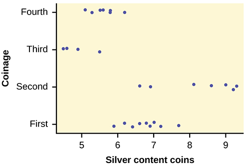
While there are differences in spread, it is not unreasonable to use ANOVA techniques. Here is the completed ANOVA table:
| Source of Variation | Sum of Squares (SS) | Degrees of Freedom (df) | Mean Square (MS) | F |
|---|---|---|---|---|
| Factor (Between) | 37.748 | 4 – 1 = 3 | 12.5825 | 26.272 |
| Error (Within) | 11.015 | 27 – 4 = 23 | 0.4789 | |
| Total | 48.763 | 27 – 1 = 26 |
P(F > 26.272) = 0;
Reject the null hypothesis for any alpha. There is sufficient evidence to conclude that the mean silver content among the four coinages are different. From the strip chart, it appears that the first and second coinages had higher silver contents than the third and fourth.
The American League and the National League of Major League Baseball are each divided into three divisions: East, Central, and West. Many years, fans talk about some divisions being stronger (having better teams) than other divisions. This may have consequences for the postseason. For instance, in 2012 Tampa Bay won 90 games and did not play in the postseason, while Detroit won only 88 and did play in the postseason. This may have been an oddity, but is there good evidence that in the 2012 season, the American League divisions were significantly different in overall records? Use the following data to test whether the mean number of wins per team in the three American League divisions were the same or not. Note that the data are not balanced, as two divisions had five teams, while one had only four.
| Division | Team | Wins |
|---|---|---|
| East | NY Yankees | 95 |
| East | Baltimore | 93 |
| East | Tampa Bay | 90 |
| East | Toronto | 73 |
| East | Boston | 69 |
| Division | Team | Wins |
|---|---|---|
| Central | Detroit | 88 |
| Central | Chicago Sox | 85 |
| Central | Kansas City | 72 |
| Central | Cleveland | 68 |
| Central | Minnesota | 66 |
| Division | Team | Wins |
|---|---|---|
| West | Oakland | 94 |
| West | Texas | 93 |
| West | LA Angels | 89 |
| West | Seattle | 75 |
Here is a stripchart of the number of wins for the 14 teams in the AL for the 2012 season.
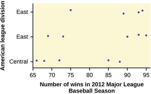
While the spread seems similar, there may be some question about the normality of the data, given the wide gaps in the middle near the 0.500 mark of 82 games (teams play 162 games each season in MLB). However, one-way ANOVA is robust.
Here is the ANOVA table for the data:
| Source of Variation | Sum of Squares (SS) | Degrees of Freedom (df) | Mean Square (MS) | F |
|---|---|---|---|---|
| Factor (Between) | 344.16 | 3 – 1 = 2 | 172.08 | 26.272 |
| Error (Within) | 1,219.55 | 14 – 3 = 11 | 110.87 | 1.5521 |
| Total | 1,563.71 | 14 – 1 = 13 |
P(F > 1.5521) = 0.2548
Since the p-value is so large, there is not good evidence against the null hypothesis of equal means. We decline to reject the null hypothesis. Thus, for 2012, there is not any have any good evidence of a significant difference in mean number of wins between the divisions of the American League.