
27 Random Forest
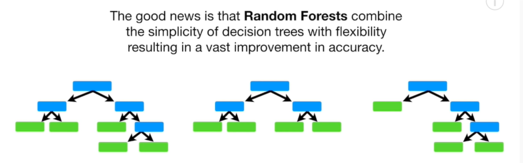
Since a single decision tree does not perform well we can have multiple trees: Random Forest!
Random Forests combine the simplicity of decision trees with flexibility in a vas improvement in accuracy.
How to build and evaluate a random forest?
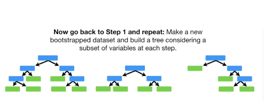
- Create a Bootstrapped data set from the original data set
- Build Trees
- Run Data Along Each Tree
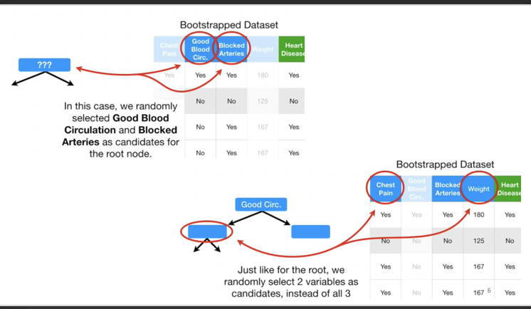
1. Bootstrap
We need to construct hundreds of trees without any pruning. After that we will learn a classifier for each bootstrap sample and average them

Bagging
Bagging can be defined as bootstrap aggregating is a method that result in low variance.
If we split the data in random different ways, decision trees give different results, high variance.
If we had multiple realizations of the data (or multiple samples), we could calculate the predictions multiple times and take the average of the fact that averaging multiple onerous estimations produce less uncertain results
Evaluating Random Forest
•Remember, in bootstrapping we sample with replacement, and therefore not all observations are used for each bootstrap sample. On average 1/3 of them are not used!
•We call them out‐of‐bag samples (OOB)
•We can predict the response for the i-th observation using each of the trees in which that observation was OOB and do this for n observations
•Calculate overall OOB MSE or classification error
Variable Importance Measures
•Bagging results in improved accuracy over prediction using a single tree
•Unfortunately, difficult to interpret the resulting model. Bagging improves prediction accuracy at the expense of interpretability.
•Calculate the total amount that the RSS or Gini index is decreased due to splits over a given predictor, averaged over all B trees.
Trees and Forests
•The random forest starts with a standard machine learning technique called a “decision tree” which, in ensemble terms, corresponds to our weak learner. In a decision tree, an input is entered at the top and as it traverses down the tree the data gets bucketed into smaller and smaller sets.
Random Forest Algorithm
•For b = 1 to B:
(a)Draw a bootstrap sample Z∗ of size N from the training data.
(b) Grow a random-forest tree to the bootstrapped data, by recursively repeating the following steps for each terminal node of the tree, until the minimum node size nmin is reached.
i.Select m variables at random from the p variables.
ii.Pick the best variable/split-point among the m.
iii.Split the node into two daughter nodes. Output the ensemble of trees.
•To make a prediction at a new point x we do:
– For regression: average the results
– For classification: majority vote
Training the algorithm
•For some number of trees T:
•Sample N cases at random with replacement to create a subset of the data. The subset should be about 66% of the total set.
•At each node:
•For some number m (see below), m predictor variables are selected at random from all the predictor variables.
•The predictor variable that provides the best split, according to some objective function, is used to do a binary split on that node.
•At the next node, choose another m variables at random from all predictor variables and do the same.
•Depending upon the value of m, there are three slightly different systems:
•Random splitter selection: m =1
•Breiman’s bagger: m = total number of predictor variables
•Random forest: m << number of predictor variables. Breiman suggests three possible values for m: ½√m, √m, and 2√m
Advantages of Random Forests
•No need for pruning trees
•Accuracy and variable importance generated automatically
•Overfitting is not a problem
•Not very sensitive to outliers in training data
•Easy to set parameters
•Good performance
Python 3 Example: Please click here to see the Python3 Example.