
Working with EIA 2014-18 Trend Data
Data Source: The data you will be working is from the U.S. Energy Information Administration (EIA) website. The EIA “collects, analyzes, and disseminates independent and impartial energy information to promote sound policymaking, efficient markets, and public understanding of energy and its interaction with the economy and the environment (Source: EIA.gov).” EIA content is often among the data sets that analysts with backgrounds in accounting, finance, supply chain, and management information systems work with in energy-related industries.
Data Context: Go to the EIA website and review information shared about Petroleum Administration for Defense Districts (PADDs). Read about the history of PADDs and how they have been used to describe movements through a variety of means of transportation (pipeline, tanker, barge, and rail) between districts today. Bookmark, save or print this page for your records in order to quickly access information and answer questions regarding PADD regions as you work with your data following the steps below.
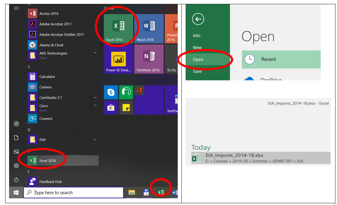
Step 2: Open your desktop copy of Excel from the Start Menu, or wherever you like to Pin the app (Start or Task Bar. Open the EIA_Imports_2014-18.xlsx file from the application.
Step 3: Observe the four worksheets in this workbook.
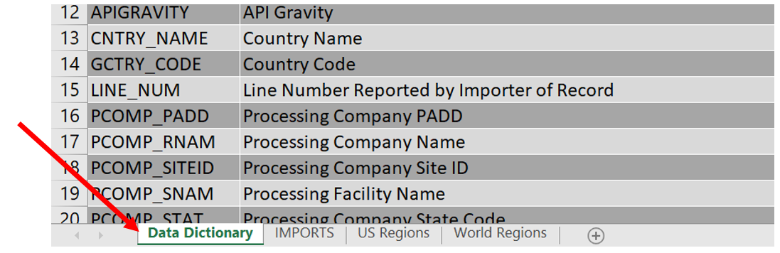
The Data Dictionary sheet contains two tables of text and notes the source of the data as well as describes what each field name (column headings) means. The meaning of some of the field names provided by the EIA is not immediately clear. Consider the PCOMP_RNAM field name and how we need to find out what entity or concept is abbreviated as such. It is a generally accepted practice to create a data dictionary or data definition table that notes what each field name means. Some abbreviations make more sense than others, checking the Data Dictionary prevents misunderstandings from occurring.
In most instances, field names will be logical and assigned with clarity, but with larger data sets, you will have to spend time to familiarize yourself with field names/column headings so that you understand what the data represents. In our case, PCOMP_RNAM refers to the Processing Company Name. Observe some of the other field names and consider how using abbreviations makes column headings narrower, our tables easier to navigate.
The IMPORTS sheet contains a large data table of text, dates, and numbers. It contains 20 columns and 122,339 rows, totaling to 2,364,880 individual data points. Consider for a moment how large Excel is despite NOT being a Big Data tool: it has over 16,000 columns (column A to column XFD) and over 1,000,000 rows. Each of these rows can contain records for over 16,000 fields. Isn’t that amazing? Note the volume of data you can squeeze into Excel, because the more you squeeze in, the more computing power you will need to process it all, the more opportunities for slower performance, errors, omissions, etc. that may impact the overall health of your hardware and the data itself.
The last two sheets in your workbook are sheets with simple tables listing US Regions and World Regions with states or countries listed next to them. You will use the contents of the IMPORTS sheet data in combination with the World and US Regions sheets to make observations about Importing or Processing Company based on the region of origin or region where ports or companies are located to serve as a higher level category above U.S. states or PADD regions.
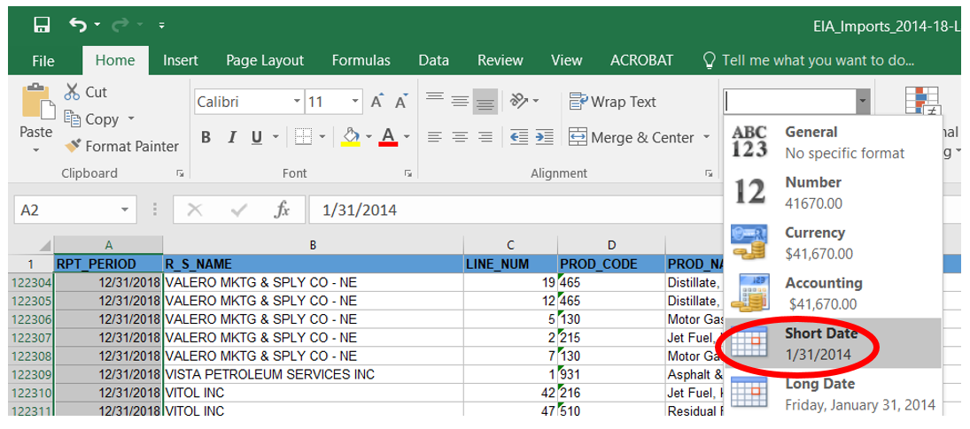
Step 4: We want to make sure that our values are used consistently across our sheet, therefore, we will edit some of the existing values that may be problematic down the line. First, we will edit the dates in column A. Go to the IMPORTS worksheet and click into the first value in the RPT_PERIOD field (cell A2). Click and hold the SHIFT+CTRL+DOWN ARROW KEY buttons to highlight the entire range of cells from A2:A122339. While this range is highlighted, go to the Number tab on the Ribbon and select the Short Date format (MM/DD/YYYY).
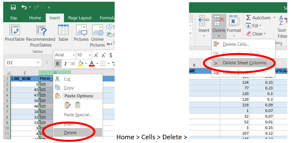
Step 5: Delete the PROD_CODE (Column D) and SULPHUR (Column M) columns, we will not be using them. You can either right click the column you wish to delete and select the Delete option from the dropdown menu OR go to Home > Cells > Delete > Delete Sheet Columns and proceed from there.
Step 6: Next, we want to make sure we have an easier time interpreting data by changing some of the field names to their Data Dictionary table names. Rename the following fields:
- R_S_Name to Importing Company Name (Column B),
- PROD_NAME (Column D) to Product Name
- PCOMP_RNAM (Column N) to Processing Company,
- PCOMP_SNAM (Column O) to Processing Facility.
You can do this manually, but that makes you prone to typos. You can accomplish the above tasks a variety of ways. You can copy and paste the definitions to replace the field names by highlighting the contents of the respective data dictionary cells, and then copy-pasting them into their new locations:
Option 1: Home > Copy/Paste options
Option 2: CYRL+C and then CTRL=V
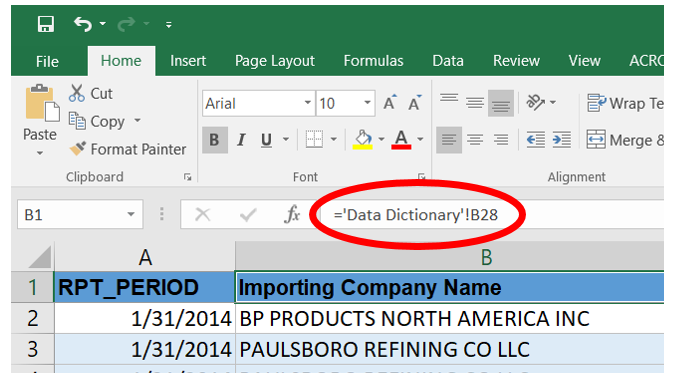
Option 3: Click into the cell where you want the data dictionary contents returned, type in an = sign, then click into the relevant data dictionary sheet cell. Importing Company is shown as reference. Observe the syntax, how the cell reference points out of the IMPORTS sheet and into Data Dictionary.
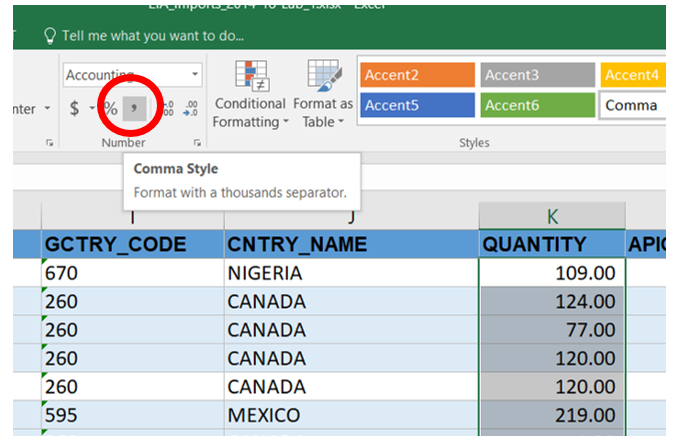
Step 7: Highlight the values under the QUANTITY field (same process as on Step 4), change the number format to Accounting number format/Comma Style.
The PivotTable feature in Excel allows us to see massive amounts of data condensed into what is a manageable format. The IMPORTS data set viewed in its raw format is difficult to summarize, understand, or take any meaningful information from. However, taking data and summarizing it in a PivotTable will allow you to manipulate and view subsets of the data in different ways. You will be able to create a structure that your or anyone can easily interpret and understand.
Previously, you have looked at the Data Dictionary and made some edits to our field names. You have also read some of the contextual information about the EIA; you should have a general understanding of what each column represents, a general idea of what types of questions you could ask of the data.
2,364,880 individual data points can give you a lot to interpret.
Using a PivotTable, you can organize, group, or totally rearrange the data in your sheet into more manageable chunks. A PivotTable will apply summary functions to our data (such as AVERAGE, SUM, MIN, MAX, and COUNT) and allows the end-user to select what view of this data that they wish to see with tools to sort, filter, and analyze these summary functions.
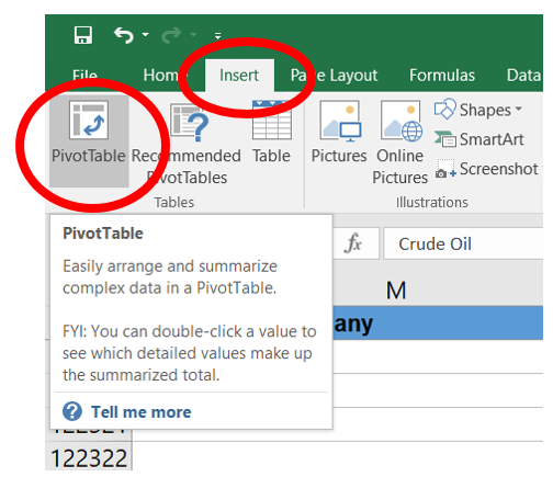
Step 8: Create a few basic summary tables using Excel’s PivotTable feature so that we can quickly get something out of our 2,364,880 individual data points in our IMPORTS worksheet. Click into cell A1. Next, insert a PivotTable based on the contents of the IMPORTS sheet into a new worksheet.
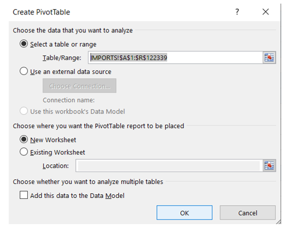
Do NOT try to select the data manually, you are not as fast as Excel. Do NOT select the contents of the entire worksheet, which would select 16,000+ columns and a million rows, likely crushing Excel in the process. Allow Excel to select the range within your worksheet with data in it. Confirm the source range as IMPORTS!$A$1:$R$122339. The absolute references in the range reference will allow for us to move this visualization/summary table into a New Worksheet.
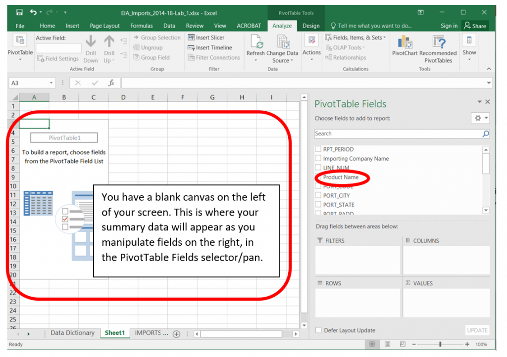
To add a field to your PivotTable, select the field name checkbox in the PivotTables Fields pane. Excel will automatically insert the field into where it feels belongs as a default area. The four options are Filters, Columns, Rows, and Values. “Non-numeric fields are added to Rows, date and time hierarchies are added to Columns, and numeric fields are added to Values” (support.office.com).
Step 9: Check the box next to the Product Name and Quantity fields in the PivotTables Fields pane. With these two clicks, Excel has summarized the Quantity imported of each of the Products from the close to 2.4 million records. Excel automatically applied the SUM function under Values to the Quantity field.
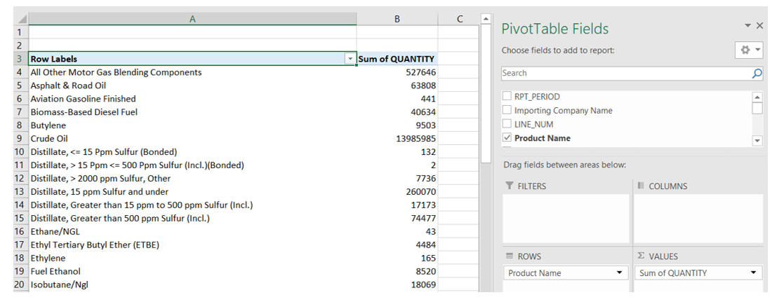
Step 10: The default output shows items in alphabetical order. You want to know what the top 5 imported products are based on the Product Name and Quantity fields. You can scroll and manually order items, but it’s generally faster to allow Excel to do the work.
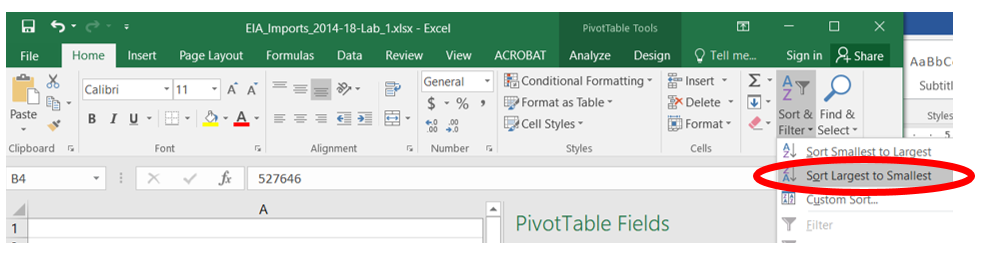
Option 1: Click into cell B4. Go to the Home > Editing tabs and select the Sort & Filter tab. Select Descending order, Sort Largest to Smallest.
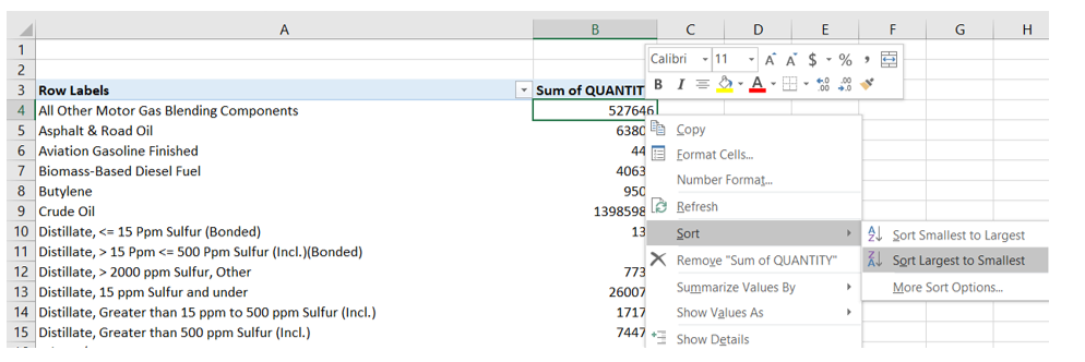
Option 2: Right-click into cell B4, select the Sort > Sort Largest to Smallest option.
Exercises
Answer the following questions based on your output after Step 10.
Question: What is the product with the highest quantity imported?
Answer: Crude Oil
Question: What is the product with the third highest quantity imported?
Answer: All Other Motor Gas Blending Components
Question: How much Jet Fuel, Kerosene-Type is imported?
Answer: 208173 (thousands of barrels)
Step 11: Next, we want to find out what percentage of all imported quantities is Crude Oil. Under Values in the PivotTable Fields pane, select Sum of QUANTITY. The Value Field Settings dialog box will pop out. Click into Show Values As. Select % of Grand Total from the dropdown.
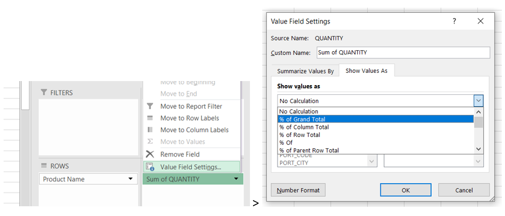
The values in column B will show as percentages.
Exercises
Answer the following questions based on your output after Step 11.
Question: What percentage of the grand total is all of the Crude Oil imported?
Answer: 77.50%
Question: How many products are there with greater than 1% of the grand total imported?
Answer: 10
Question: What percentage of the grand total is all of the Asphalt & Road Oil imported?
Answer: 0.35%
Step 12: Next, we want to find out what percentage of all imported quantities of Crude Oil arrives into the state of Texas. Keep the fields as it from the previous step and click the PORT_STATE field. Excel will place the new field under the Product Name field under the ROWS pane.
Exercises
Answer the following questions based on your output after Step 12.
Question: What percentage of all of the Crude Oil imported into the United States arrives into Texas?
Answer: 18.07%
Question: Which state receives the second highest % of all the Crude Oil imports in the United States?
Answer: Illinois
Question: Which state sees a higher % of the Crude Oil Imports? California or Louisiana?
Answer: Louisiana
Step 13: Next, we want to find out what % of all the products quantities that arrive into Texas is Crude Oil and other products. Drag the PORT_STATE field from ROWS to under the FILTERS area. You will see the PORT_STATE filter appear in the top right corner of your worksheet. Select TEXAS from the dropdown in cell B1.
Exercises
Answer the following questions based on your output after Step 13.
Question: What percentage of all of the products that arrive into port state Texas are the Crude Oil quantities?
Answer: 82.99%
Question: Which product has the second highest % of all imports into the state of Texas?
Answer: Unfinished Oils, Heavy Gas Oils
Question: What percentage of all of the products that arrive into port state Illinois are the Crude Oil quantities?
Answer: 99.69%
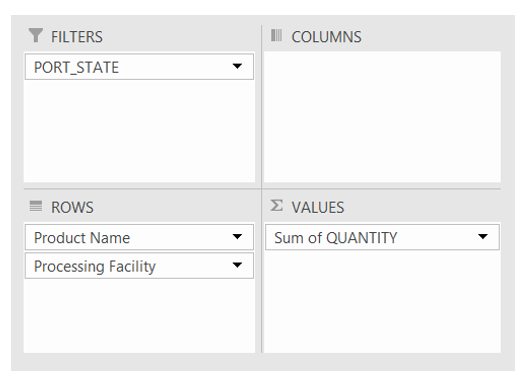
Step 14: Next, we want to find out which Processing Facility in the PORT_STATE of Texas processed the highest % of Crude Oil. Set the PORT_STATE filter back to TEXAS. Drag the Processing Facility field name under ROWS. Sort your Sum of QUANTITY Column in descending order.
Exercises
Answer the following questions based on your output after Step 14.
Question: What percentage of Crude Oil quantities arrive into PORT ARTHUR?
Answer: 26.79%
Question: Which facility has the second highest percentage?
Answer: BAYTOWN
Question: What percentage of Crude Oil quantities arrive into BEAUMONT?
Answer: 1.93%
