
Chapter 8: Fossils and Paleoenvironments
Learning Objectives
The goals of this chapter are to:
- Categorize fossil assemblages to determine their habitats
- Develop connections between modern and ancient paleoenvironments
- Evaluate paleoenvironments through time and space
8.1 Introduction
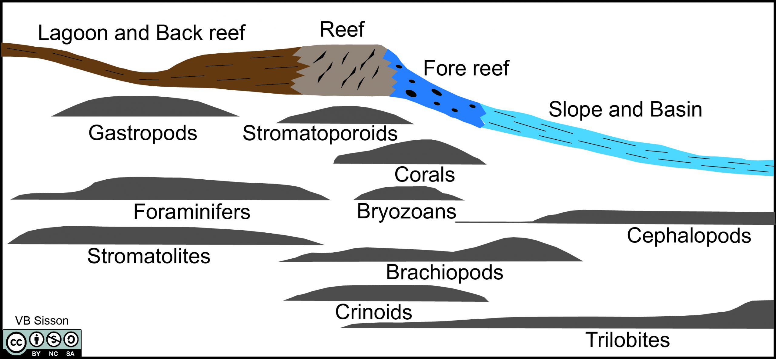
Some geologists use fossils to determine stratigraphy and correlate stratigraphic sequences. Others prefer to study paleoecology to determine ancient habitats where both plants and animals co-existed. This avenue leads to discoveries about past climate, predator-prey relationships, and even ocean depth. Using this information, artists create reconstructed paleoenvironments (Figure 8.1) to display these ancient habitats.
Remember, fossils are not just exciting curiosities but were once living organisms that reproduced, ate each other, and interacted with their environment just like we do. A fossil’s paleoecology depends on many factors of their paleoenvironment. These include physical conditions, such as temperature, light, water depth, and energy (calm vs. turbulent), and chemical conditions, such as salinity, pH, oxygen, and toxic chemicals. Some animals will thrive if these variables change, and others will die off. Have you ever been to the beach and seen large piles of seaweed? They came from the middle of the ocean and were brought to shore as ocean currents and winds changed. Some organisms can survive environmental change, such as oysters that can live in both salty and freshwater. Fossils hold the key to determining what the paleoenvironment was like. This ability to reconstruct a fossil’s paleoenvironment is one of the most valuable tools that a paleontologist has to offer to broader fields in geology.
Exercise 8.1 – Devonian Reef
Head to the PaleoDB Navigator. A large map of the world should open with many colored circles. The circles represent locations where fossils have been discovered, and the color of the circle corresponds to the geologic timescale at the bottom of the page. You can click through the different time periods to see where fossils of that age have been discovered. On the right side, there is a list of the most abundant fossil groups based on the time period you have selected on your map view. For example, you could zoom in on fossils found in South America from the Ordovician Period. The menu on the right will update with what fossils are found on your map for that period. Depending on your zoom level, you may see that the Trilobita Class is the most abundant, or you may see it broken down into several orders of Trilobita with the Asaphida Order as the most abundant. If there is lower diversity of fossils in your map view and time period, you will see the classification broken down to lower levels. You may find you need to Google some of the names to figure out what phylum, class, or order they belong to. You can clear whatever filters you select on the lower left side of the page.
- In the PaleobioDB Navigator, set your time period to Devonian and zoom in on New York State. What is the most common group of Devonian fossils found in New York? Remember, you may need to search more technical taxonomic names to determine which fossils you’re looking at (I’m talking about you, Rhynchonellata and Strophomenata).
- What are some other organisms that are present?
- What type of environments are most of these organisms found in?
- Compare the locations of gastropods and cephalopods. You can do this by clicking on the classes on the right-hand menu. Look at the two locations of these fossils compared to each other. You may find it easier to have two browser windows open for this. Based on the locations from the navigator and the typical locations of fossils around a Devonian reef, what direction was the coastline located?
- Remove any organism filter and now look at the distribution of all fossils throughout the Devonian in New York. Click on “E”, “M”, and “L” under Devonian to look at the distribution from early to middle to late Devonian. Was sea level rising or falling in this region during the Devonian (you already know which way the coastline was based on your previous answer)?
Exercise 8.2 – Himalayan Mountains
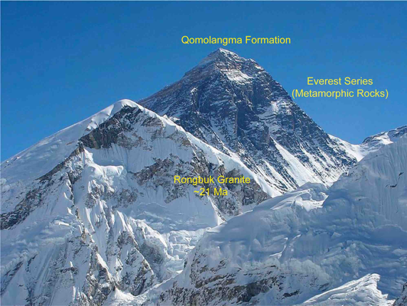
- Figure 8.3 shows the tallest peak on Earth, Mount Everest, at 8,848 m (29,029 ft) (Tibetan name Qomolangma). It has a layer of unaltered limestone from the Ordovician at its summit. What does this tell you about the environment of Mt. Everest during that time?
- Using the PaleoDB navigator, look at the distribution of fossils for the Himalaya Mountains, particularly near the Nepal/China border. During which two geologic time periods were fossils most abundant?
- What were the most abundant organisms for each of those periods? The pane on the right side tells you the percentage of each organism found in your current map view. You may need to search the technical taxonomic name to learn which organism it is.
- Based on the changes in fossils over the time periods, determine whether sea level was rising, falling, or constant. Be sure to explain your answer.
- Critical Thinking: Does your sea-level interpretation match the global sea-level record from Figure 5.21? Explain your answer.
Exercise 8.3 – Western Interior Seaway
The Western Interior Seaway, also called the Cretaceous interior seaway, was a large, shallow sea during the Late Cretaceous that split the North American continent into two pieces.
Head back to the PaleoDB Navigator. Zoom in so that the United States takes up most of the map, and then select the Late Cretaceous as your time period.
-
- Describe the distribution of all fossils during the late Cretaceous in the U.S., particularly in the central-western part of the country (Texas to Montana).
- What is the most abundant group of fossils found during this time period? ____________________
- Based on the fossils present and their location, describe what the environment would have been like.
- Describe the distribution of all fossils during the late Cretaceous in the U.S., particularly in the central-western part of the country (Texas to Montana).
Exercise 8.4 – Interpreting Paleo-Water Depth
Foraminifera, informally called forams, are tiny, single-celled marine organisms about the size of a grain of sand. They come in two broad varieties, benthic (living on the ocean floor) and planktonic (floating in the water column). Forams build a shell, called a test, mainly out of calcium carbonate. When forams die, their shells can be deposited as sediment on the ocean floor and can be recovered during scientific drilling expeditions, as discussed in Chapter 5.
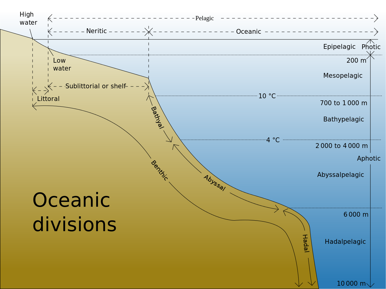
Forams are sensitive to seawater characteristics, like temperature, salinity, water depth, etc., and each species has a set range of seawater characteristics in which they live. For this exercise, we will use forams to interpret paleo-water depth. Below is a list of five species of forams and their preferred water depth range. Figure 8.4 shows the divisions of the ocean based on water depth. For a full description of these divisions, see Introduction to Oceanography by Paul Webb.
- Cibicidoides mundulus – Bathyal to abyssal
- Cibicidoides wuellerstorfi– Bathyal
- Gyroidinoides soldanii – Mesopelagic to bathyal
- Nuttallides umbonifera – Lower bathyal to abyssal (corrosive water)
- Oridorsalis umbonatus – Widely distributed
You are assuming the role of a micropaleontologist. During a recent scientific drilling expedition, you collected sediment samples from five sections of a sediment core. You want to determine the water depth when each layer of sediment was deposited using foram fossils. You’ve identified all of the species of forams present and their abundance for each sample.
- Sometimes, looking at data in terms of a percentage rather than the raw numbers makes data easier to interpret. Convert the raw numbers of forams in each sample (Table 8.1) to a percent (Table 8.2). Sample 1 is already done for you.
Table 8.1 – Numbers of foram species per sediment sample Foram Species (numbers) S1 S2 S3 S4 S5 C. mundulus 83 107 0 52 8 C. wuellerstorfi 91 0 0 69 0 G. soldanii 82 0 157 58 77 N. umbonifera 30 143 0 76 72 O. umbonatus 44 84 100 54 38 Total 330 Table 8.2 – Percentage of foram species per sediment sample Foram Species (percent) S1 S2 S3 S4 S5 C. mundulus 25% C. wuellerstorfi 28% G. soldanii 25% N. umbonifera 9% O. umbonatus 13% Total 100% - Using Figure 8.4, determine the pelagic zone and depth range for each sediment sample in Table 8.3. Sample 1 is already done for you.
Table 8.3 – Pelagic zone and depth range of sediment samples Sediment Sample Pelagic Zone Depth Range S1 Bathyal 700 – 1000 m S2 S3 S4 S5 - If sample 5 is the oldest and sample 1 is the youngest, describe how the water depth changed through time.
This exercise is adapted from Steve Pekar, Queens College, City University of New York.
8.2 Fossils and Paleoenvironments in Movies
We all know that Hollywood stretches the truth (or outright makes it up) when depicting science in movies. Perhaps the most famous movie depicting fossils and paleoenvironments is the Jurassic Park series. For example, in the original movie from 1993, there is a scene where a Tyrannosaurus rex chases a Jeep at over 60 mph. At the time of production, some paleontologists thought T. rex could only run at a maximum speed of about 45 mph. However, we now know that T. rex didn’t have the hip structure to support running and was more of a brisk walker. So, you could probably outrun a T. rex.
Exercise 8.5 – Jurassic Park
Using the PaleobioDB Navigator, look up “Dinosauria” (an unranked clade). A clade is a group of organisms that share a common ancestor, and cladistics is a way to classify organisms based on common characteristics. You’ll notice that one of the groups in the Dinosauria clad is Aves, which is the class comprising birds. Yes, according to cladistics and taxonomic rankings, dinosaurs and birds are related.

- During which range of geologic time periods were Dinosauria most abundant (excluding Aves)?
- Which one of those time periods were Dinosaurs (not Aves) most abundant?
- The movie franchise Jurassic Park showcases several different dinosaurs. The table below contains the seven dinosaur genera shown in the original film from 1993. Complete the table below with what geologic time periods these dinosaurs lived and what their preferred habitat was (use Google to search for the “[genera] habitat.” Remember, the movie depicted all of these dinosaurs living in a tropical climate.
Table 8.4 – Worksheet for Exercise 8.4. Genera Geologic Time Period Preferred Habitat Tyrannosaurus Brachiosaurus Triceratops Velociraptor* Dilophosaurus Gallimimus Parasaurolophus *In the movies and book Velociraptor was based on a similar dinosaur, called Deinonychus, in almost every detail, and only the name had been changed to be more dramatic.
- Jurassic Park was primarily filmed in Hawaii. Do you think all of the dinosaurs could survive in that tropical environment?
- Does Jurassic Park seem like a fitting name based on when these dinosaurs lived? Why or why not?
Additional Information
Exercise Contributions
Daniel Hauptvogel and Virginia Sisson
Exercise 8.1 was inspired by an exercise on Life Mode Characteristics by Steven J. Hageman at Appalachian State University
References
Barreda V.D., Cúneo N.R., Wilf P., Currano E.D., Scasso R.A., Brinkhuis H., 2012, Cretaceous/Paleogene Floral Turnover in Patagonia: Drop in Diversity, Low Extinction, and a Classopollis Spike. PLoS ONE 7(12): e52455. https://doi.org/10.1371/journal.pone.0052455
Corradini, C., Pondrelli, M., Corriga, M.G., Simonetto, L., Kido, E., Suttner, T.J., Spalletta, C., and Carta, N., (2012). Geology and stratigraphy of the Cason di Lanza area (Mount Zermula, Carnic Alps, Italy). Berichte des Institutes für Erdwissenschaften, Karl-Franzens-Universität Graz. 17. 83-103.
Google Earth Locations

the natural home or environment of a plant or animal
an environment that prevailed at some time in the geologic past
a group of organisms believed to have evolved from a common ancestor

.jpg)