Chapter 2: Topographic Maps

Daniel Hauptvogel; Virginia Sisson; Michael Comas

Chapter 2: Topographic Maps

Latitude, longitude, directions, and contour lines

Learning Objectives

The goals of this chapter are to:

Understand different map features
Interpret topographic lines
Explain topographic maps and profiles

2.1 Map Basics

Maps are to a geologist like a wrench is to a mechanic or paint is to an artist. They’re an integral part of studying the Earth and are used by just about every type of geoscientist. Geologists use maps to visualize data over an area, such as elevation, rock type, groundwater level, hazards, pollution, etc. Oftentimes, maps depict 3-dimensional features in a 2-dimensional space, and inexperienced map readers can have a tough time visualizing this.

Exercise 2.1 – Connecting 3D features on a 2D Map

Your instructor will bring you to the augmented reality sandbox.

Recreate the topographic map from Mt. Guyot, California (Figure 2.1) in the augmented reality sandbox.
Describe the contour lines pattern representing the top of Mt. Guyot.
Describe the pattern of the contour lines that represent the Guyot Flat.
Figure 2.1 shows two streams (blue lines). Describe what happens to contour lines when they cross streams.
Which way do you think is downstream?
Critical Thinking: This mountain is named after a famous Swiss geologist, Arnold Guyot, who was one of the first to describe the motion of glaciers. The term guyot is also used to describe a flat-topped underwater volcano with a summit that can be up to 6 km across. Describe any features similar to a marine guyot.

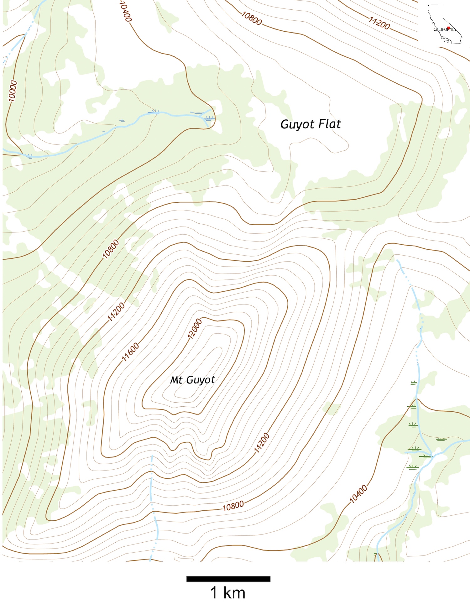
Figure 2.1 – A topographic map of Mt. Guyot, California. Elevation is in feet. Image credit: adapted from the USGS Mount Whitney Quadrangle, Public Domain.
Flatten the sand in the box to start over. Create a ridge (a narrow, linear mountain) with the sand. Make one side of the ridge shallow and the other steep. On Figure 2.2, sketch what the contour lines look like and identify your shallow side and steep side.
Locate and label the top of the ridge on your sketch in Figure 2.2.

Figure 2.2 – Sketch area for questions g and h.

Exercise 2.2 – Understanding 3D features

Your instructor will give you two three-dimensional models of the Big Island of Hawaii; a geological wonder shaped by millions of years of volcanic activity. It is home to Mauna Kea and Mauna Loa, two of the world’s largest volcanoes. Other topographic features are new lava flows, volcanic craters, deep canyons, volcanic cinder cones and popular beaches. You will either look at a 3D printed model or a computer-generated 3D model. 3D printing involves creating layers of equal thickness similar to contour lines.

1. Describe the general shape of the Big Island.
2. Now look at the two prominent volcanos Mauna Kea (4,205 meters or 13,796 feet) and Mauna Loa (4,169 meters or 13,677 feet). One of these is considered the world’s largest volcano. The other is the highest point in the state of Hawaii. How do you identify which volcano is the highest? Why is Mauna Loa considered to be a larger volcano when it is not as high?
3. In addition, there are three other volcanos on the Big Island; Hualalai, Kilauea, and Kohala. One of these is extinct and will never erupt again, one is dormant (inactive) and may erupt again, and one is active and may be erupting as you do this exercise. How do you distiguish between these three types of volcanos?
4. If you have the two different 3D printed models, describe their differences.
5. Create a simple topographic map on Figure 2.3 with several contour lines to showing the five volcanos and two major canyons on Hawaii. On your map, identify the active, inactive, and extinct volcanos. Also, indicate where on this map you predict the best beaches.
  
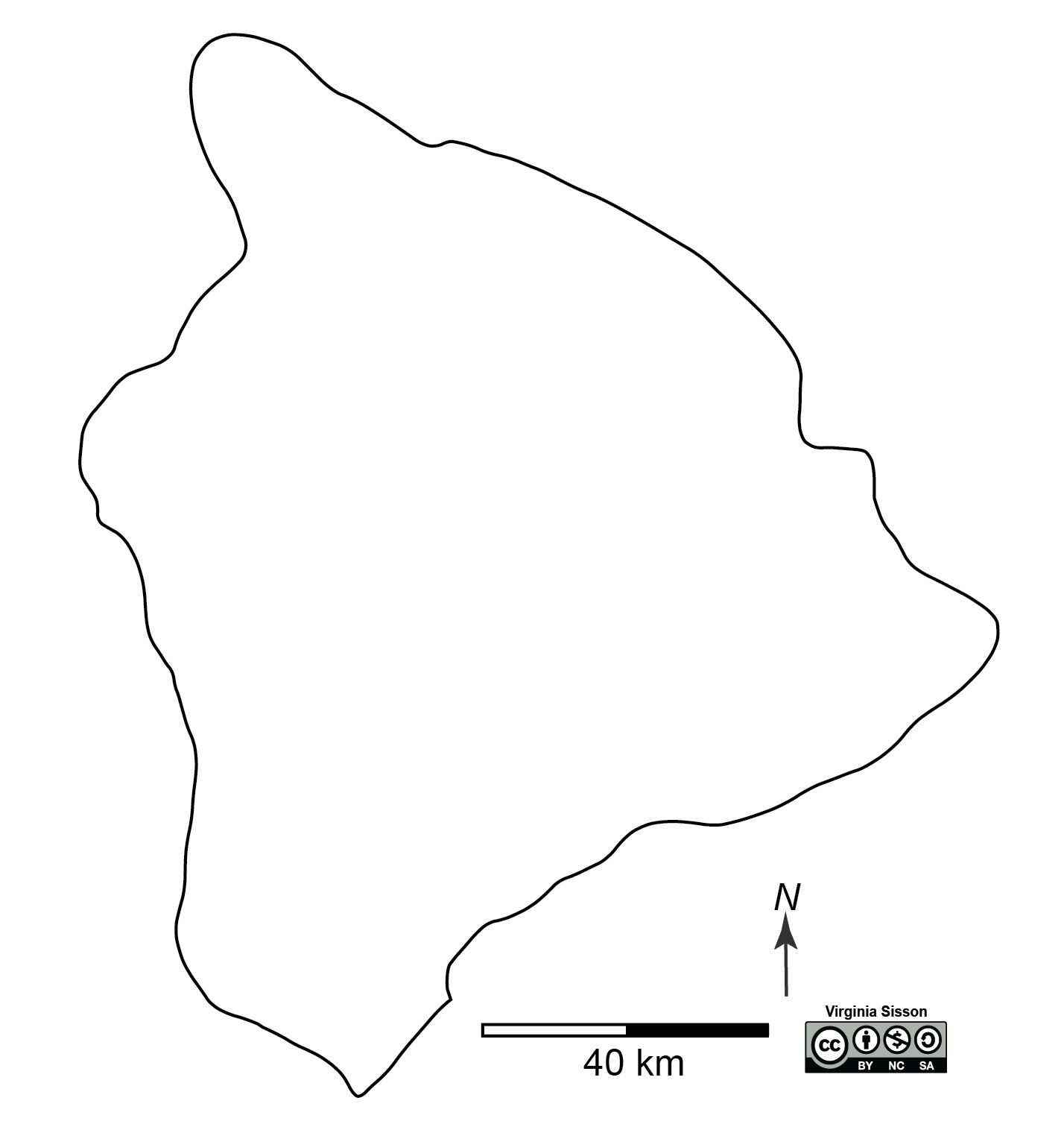
  Figure 2.3 Outline of Big Island, Hawaii to use for topographic sketch. Image credit: Virginia Sisson CC BY-NC-SA.
6. Critical Thinking: Most people either live in Hilo or Kailua-Kona on the Big Island of Hawaii. One of these is the center of tourism and the other of commercial activity. Can you identify where these are on your map? Describe the topographic features that make these locations good for tourism and commerce.

Even with all the different types of data that can be displayed, maps should all have a few things in common. Every map should have a compass to help indicate direction, a scale and scale bar to get a sense of distance, and latitude and longitude coordinates so you know where on Earth the map is located. If a map doesn’t have a north arrow, assume north is the top of the map.

The Compass

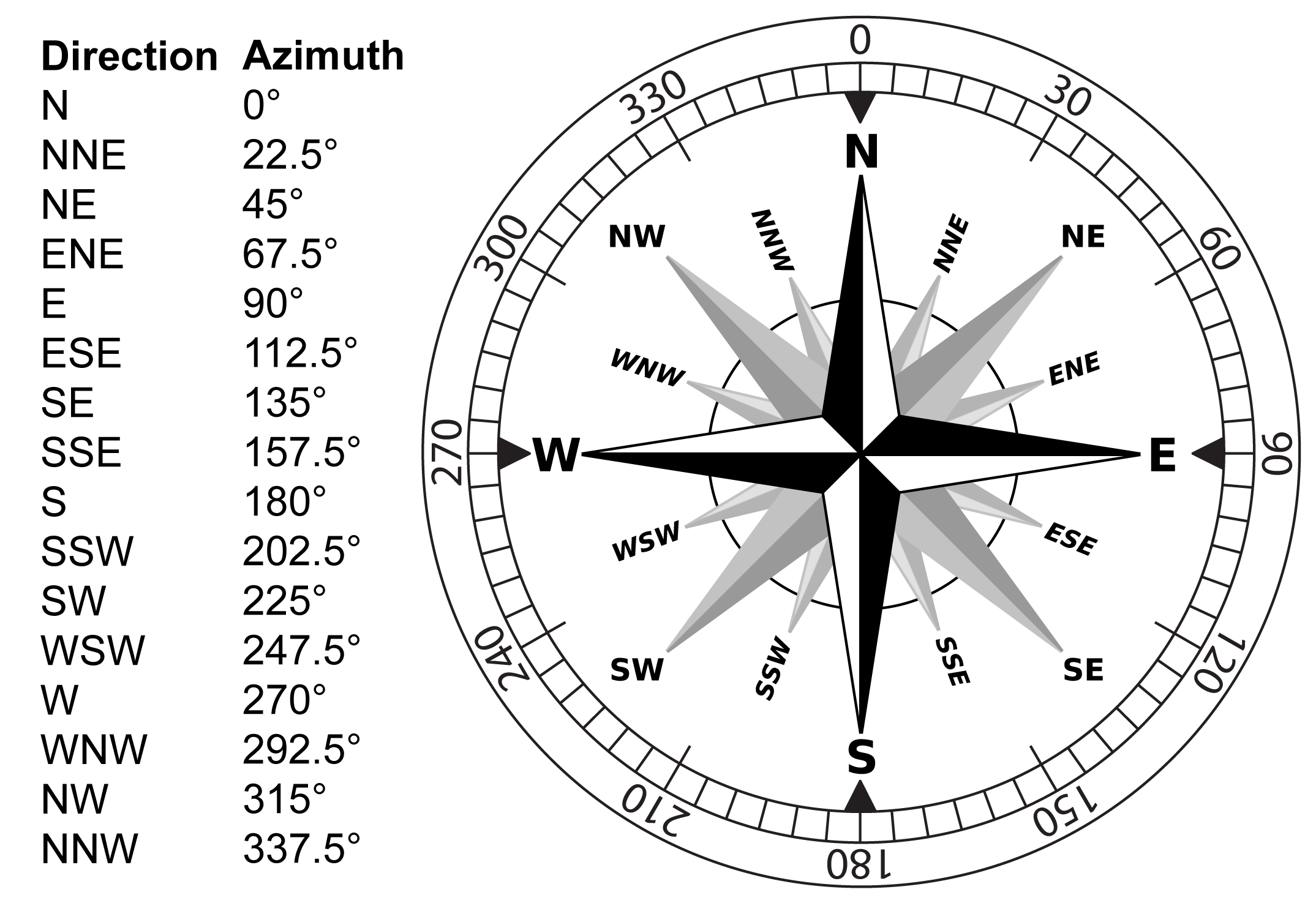
An important part of reading maps is understanding how to use a compass and recognize directions. As a geologist, you may want to know the direction a rock unit is oriented, the direction from one mountain peak to another, or the direction a paleo-river used to flow. There are two forms of direction that you should be familiar with: the cardinal directions and the azimuth system (Figure 2.4). Cardinal directions refer to north, east, south, and west and can be divided even further into intercardinal (NE, NNE, ENE, etc.). Generally speaking, when we say something is to the north, we don’t always mean that it is directly north. It’s more likely a little bit northeast or northwest. That’s where azimuth comes in. Azimuth is the angular measurement from a compass, from zero up to 360°.

Azimuth compass showing directions and corresponding degrees. — Figure 2.4 – Compass directions using cardinal and azimuth systems. Image credit: Daniel Hauptvogel and Michael Comas, CC BY-NC-SA.

Exercise 2.3 – Exploring Compass Directions

Practice your directions by using the cardinal and azimuth systems to answer the following questions.

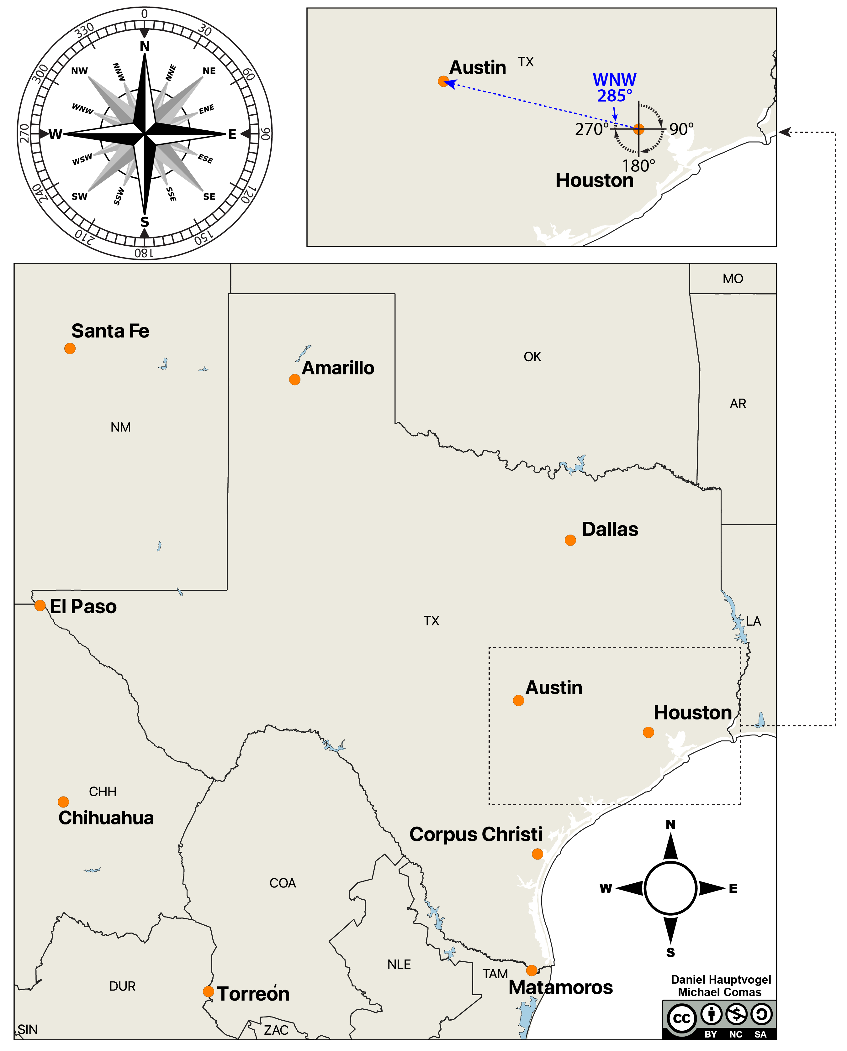
Without using a protractor, what is the cardinal direction (NW, WNW, E, SE, etc.) between the following cities in Figure 2.5 (Houston to Austin example completed for you)?
1. Houston to Austin: WNW
2. El Paso to Santa Fe: ____________________
3. Santa Fe to Dallas: ____________________
4. Dallas to Torreon: ____________________
5. Torreon to Matamoros: ____________________

Follow the steps below to find the direction (azimuth) between cities in Texas in Figure 2.5. An example has been provided along with the steps for determining the azimuth from Houston to Austin.

Use a straight edge to draw a line between your two points
Place the cross of the protractor on your starting point and orient the 90° mark on the protractor towards the north if the second point is to the north or towards the south if the second point is to the south.
Determine how many degrees away from 0 your line is pointing.

Now, use a protractor and find the azimuth directions for the cities below (Houston to Austin example completed for you).
1. Houston to Austin: 285°
2. Matamoros to Austin: ____________________
3. Austin to Chihuahua: ____________________
4. Chihuahua to Amarillo: ____________________
5. Amarillo to Houston: ____________________

Map of Texas, Oklahoma, and parts of Mexico and New Mexico — Figure 2.5 – Map showing the locations of major cities in Texas and northern Mexico. Inset map is an example of using a protractor to determine azimuth compass direction. Image credit: Daniel Hauptvogel and Michael Comas, CC BY-NC-SA.

Map Scales

Maps are scaled-down versions of the areas they represent. The word “scale” refers to the amount of reduction the map represents. All maps include at least one type of map scale to indicate the relationship between the area on the map and the area of the region it represents in reality. Map scales are provided so that a map reader can determine exactly how much distance is actually represented on their map, or to measure the distance between two points on a map, or even to calculate the gradient (slope) of a hill, valley, or river. Map scale is represented by a fraction, graphic scale, or verbal description.

The two commonly used map scales on a topographic map are the bar scale and the fractional scale (also known as the ratio scale). The length of the bar represents the actual distance covered on the map. A standard ratio scale used in American topographic maps is 1:24,000, which means that 1 unit of measurement on the map is 24,000 units in reality (Figure 2.6). Each bar is a graphical representation of distance on the map, and you get to decide if you want to measure distances in kilometers, meters, miles, or feet. To find the distance between any two points on a map, use a piece of paper to transfer the two points down to the bar scale and read the distance directly from the bar scale. Notice that each bar scale has the starting point (zero) within the scale, and not at its beginning.

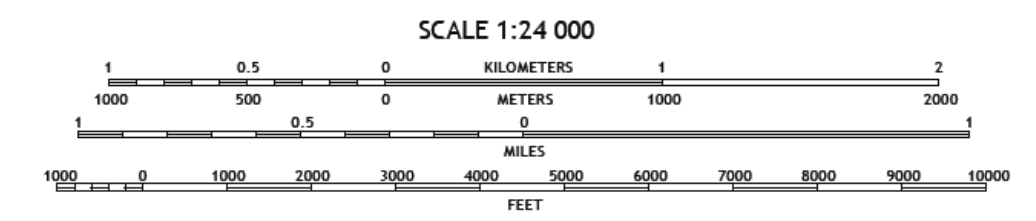
1:24,000 Scale bar — Figure 2.6. Example of a scale typically found on the bottom of a topographic map. Image Credit: Elizabeth Johnson CC SA.

In Canada and Mexico, the standard scale is 1:50,000. The unit does not matter because the principle works the same for all units; it could be inches, feet, meters, kilometers, etc. When we talk about large- and small-scale maps and geographic data, we refer to the relative sizes and levels of detail of the features represented in the data. In general, the larger the map scale, the more detail is shown.

Another way to use map scales is as fractions. For Figure 2.6, 1″ on a map equals 12,000 inches in reality. Remember that 12 inches is one foot. So, then you need a fraction 12,000 ÷ 12 = 1,000 feet. Or if you are using metric scales such as 1:40,000, 1 cm on your map = 40,000 cm in reality, or perhaps 5 cm on your map is 200,000 cm (5 x 40,000 cm) in reality. Again, remember that 100 cm = 1 m. Therefore, 200,000 ÷ 100 = 2,000 m.

Another map concept to explore is vertical exaggeration (VE). Simply put, this is a scale used in raised-relief maps, plans and technical drawings (cross section perspectives), and geological cross-sections to emphasize vertical features, which might be too small to identify relative to the horizontal scale.

The vertical exaggeration is calculated as VE = VS ÷ HS where VS is the vertical scale and HS is the horizontal scale.

Exercise 2.4 – Using Map Scales

You can use your knowledge of scales to estimate distances on maps.

On a map with a scale of 1:24,000, how long is a stream (in feet) that measures 1 inch on the map? ____________________
On a map with a scale of 1:50,000, how long is a road (in meters) that measures 5 cm on the map? ____________________
Your instructor will provide you with two maps of the Galveston, TX region at different scales. One was published in 1983, the other in 2022. What are the scales of each map?
Look closely at both maps. What information is given on the 2022 map that isn’t on the 1983 map, and vice versa?
On the northeast side of the 2022 map, measure the channel width between Galveston Island (Fort Point) and Point Bolivar. How wide is the channel on the map (cm) and in reality (m and mi)?
Do the same measurements using the map from 1983.
Which map is better for determining this distance? Why?
These maps were published 39 years apart. Can you think of any reason why this may have affected your measurements?
Do you think it is important that maps be updated often? Should certain geographic regions be re-mapped more often than others? Why?
Which map would be best to use to show the projected approach of a hurricane toward the Texas coast? Why?
Which map would best display detailed hurricane evacuation routes off of Galveston Island. Why?
Which map should a cruise ship captain use to help guide him into the port at Galveston? Why?

Coordinate Systems

An important part of geologic field work is noting the precise locations of samples, outcrops, geologic features, etc. If you or other scientists cannot return to find your location, then the data cannot be reproduced. Part of being a scientist is creating reproducible data, experiments, locations, etc.

In Chapter 1 you briefly explored the different coordinate systems for maps: Degree Minutes Seconds (DMS) and Decimal Degrees (DD). Which system you use may depend on how you keep track of your study sites. That means it’s important to not only understand different coordinate systems but also be able to convert coordinates between systems.

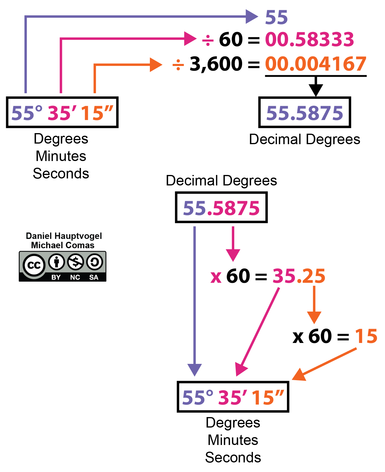
DMS divides the roughly spherical planet Earth into 360 slices that are each 1°, each degree is broken down into 60 smaller slices called minutes, and each minute is broken into 60 smaller slices called seconds. DD converts the three numbers used to define a coordinate with DMS into a single number.

Exercise 2.5 – Converting Geographic Coordinates

Figure 2.7 shows you how to convert a single coordinate back and forth between degrees, minutes, and seconds (DMS) and decimal degrees (DD).

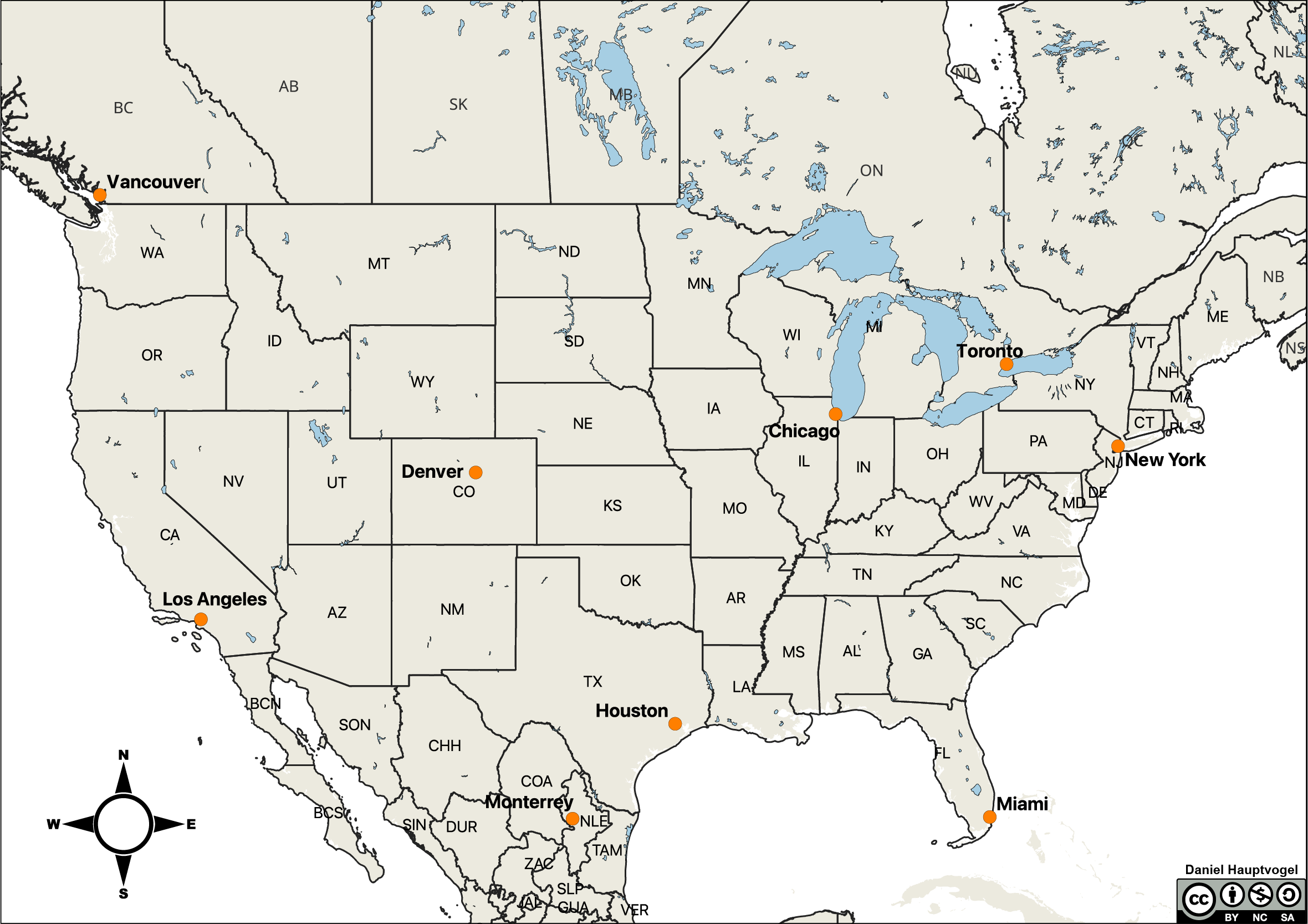
Schematic for conversion of geographic coordinates — Figure 2.7 – Flow chart for converting geographic coordinates between DMS (degrees, minutes, seconds) and DD (decimal degrees). Image credit: Michael Comas and Daniel Hauptvogel, CC BY-NC-SA 4.0.

Most GPS measurements using either a standalone instrument or an app are given in DD. But, many maps use DMS. So, it is important that you can convert between these two systems. For example, a pilot going between the major cities in North America (Figure 2.8), may have an aviation map in DMS with a DD instrument in their plane. Table 2.1 contains geographic coordinates for some cities, as shown in Figure 2.8. One of the coordinate systems is given for each city. Using Figure 2.7, convert coordinates to either DMS or DD. Denver, CO has been done for you.

Table 2.1 – Cities and their geographic coordinates
	Degrees Minutes Seconds (DMS)	Decimal Degrees (DD)
Denver, CO	39° 44′ 21″ N, 104° 59′ 25″ W	39.7392 N, 104.9903 W
New York, NY	40° 42’ 46” N, 74° 00’ 22” W
Los Angeles, CA		34.0549 N, 118.2426 W
Monterrey, Mexico		25.6866 N, 100.3161 W
Chicago, IL	41° 51’ 55” N, 87° 37′, 40” W
Houston, TX	29° 45’ 46” N, 95° 22’ 59” W
Toronto, Canada		43.6532 N, 79.3832 W

Which coordinate system do you think is better and why?

Map of the United States, southern Canada and northern Mexico. Several major cities are marked with orange circles. — Figure 2.8 – Map of the United States showing the location of five cities. Image Credit: Daniel Hauptvogel, CC BY-NC-SA.

2.2 Contour Lines and Topographic Maps

Topographic maps show the shape (topography) of the landscape, including hills, mountains, valleys, rivers, etc. These maps contain contour lines, which are lines of equal elevation. That means everywhere along that line will have the same elevation.

Elevations for major contour lines are typically marked on the line. To avoid clutter, not every contour is labeled. The elevation of an unlabeled contour line can be determined by knowing the contour interval and looking at adjacent contour lines. The elevation of a point located in between two contour lines can be estimated by interpolating between the lines. If a point is halfway between two contour lines, it will be about halfway between the elevations of those two contour lines.

In the US, topographic maps have elevation marked in feet or meters above mean (average) sea level. International maps and maps of elevation of the ocean floor (bathymetry) are usually marked in meters.

Exercise 2.6 – Contour Lines and Topographic Maps

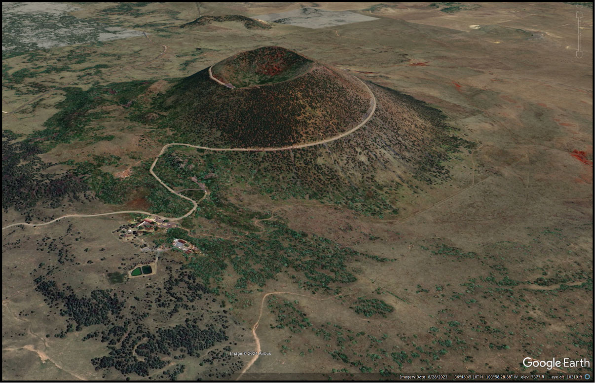
Capulin Volcano in New Mexico (Figure 2.9) is a volcanic cinder cone that is about 60,000 years old. Figure 2.10 is a map view and topographic map of the volcano.

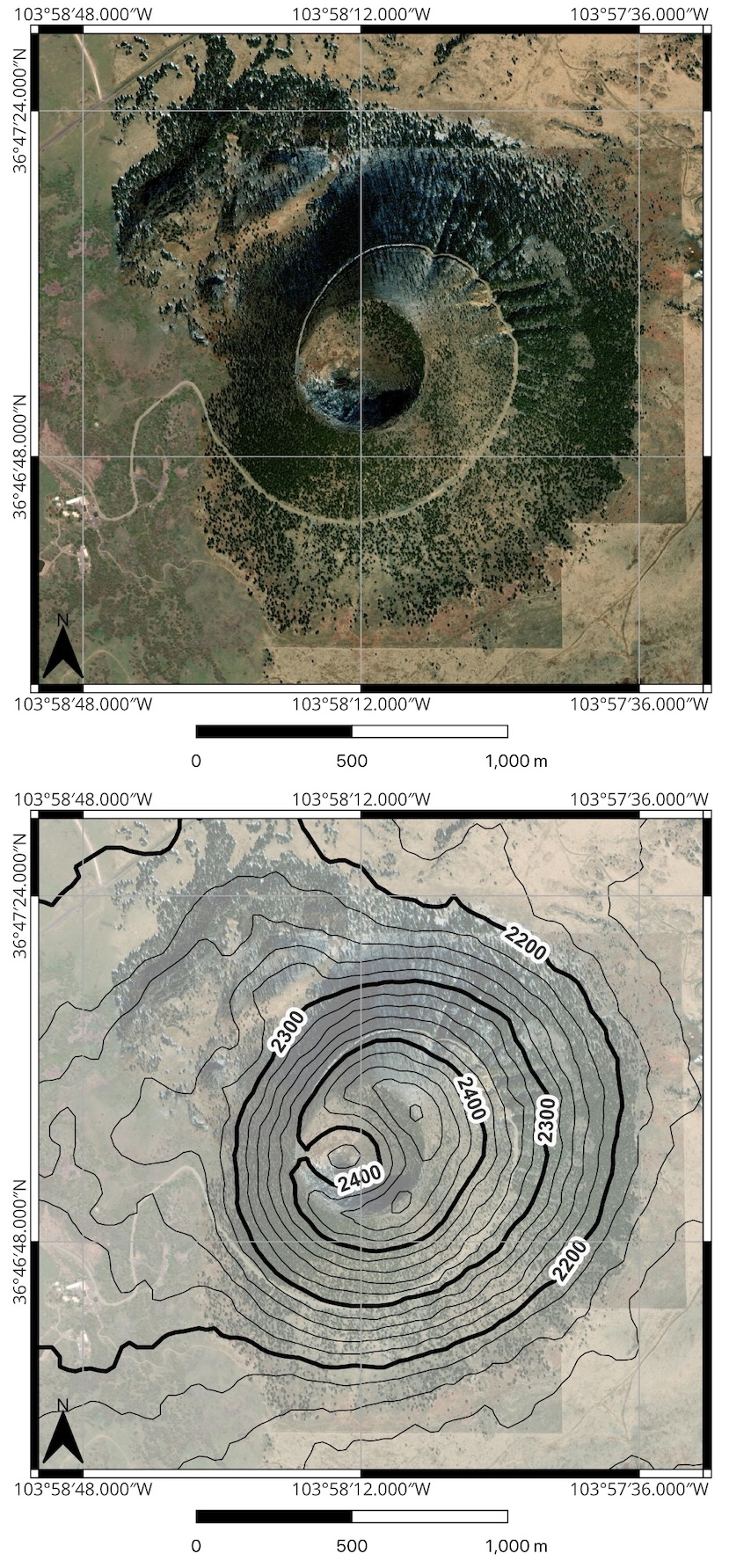
View of Capulin Volcano — Figure 2.9 – Side view of Capulin Volcano in New Mexico. Image credit: Google Earth

Top: Satellite view of Capulin volcano. Bottom: Topographic map of Capulin volcano overlayed on the satellite image. — Figure 2.10 – A: Map view of Capulin Volcano. B: Topographic map of Capulin Volcano. Image credit: Google Earth and USGS.

What pattern do you notice in the contour lines that represent the volcano?
A contour interval is the elevation difference between contour lines. Some lines are bold; these are major contours and are marked at regular intervals. On this map, the major contours are 50 m apart. What is the contour interval of this map? ____________________
What is the elevation of the highest point of Capulin Volcano? ____________________
From the highest point, how deep is the crater of the volcano? ____________________
If you either walk or drive from the visitor’s center to the scenic overlook, how much would your elevation have changed? ____________________
Topographic maps also give you a sense of the slope of the landscape. Examine the eastern and western sides of Capulin Volcano. Which side is steeper, and which is shallower? What does the spacing of the contour lines tell you about the slope?
Construct a topographic profile of this area in Google Earth Pro. Your instructor will help you.
Critical Thinking: The road to volcano crater was built by the Depression Era Civil Work Administration (CWA) in 1933-1934. Why did they pick this route?

Rules

The rules inherent in topographic maps are pretty simple: contours represent lines of equal elevation, contours always close (except on the edge of a map), contours rarely cross, closely spaced contours represent steepness, and the geometry of contours changes in predictable ways between features such as valleys and ridges. When contour lines cross a river or valley, the line forms a “V” shape. This is called the Rule of V’s.

Exercise 2.7 – Exploring Rules of Contour Lines

Below is an image from the high peaks of the Sierra Nevada and a simplified topographic map of this area. Use these to discover some other rules of topographic maps. Examine the photo and map in Figures 2.11 and 2.12.

Photo of Tulainyo Lake, California — Figure 2.11 View of Tulainyo Lake from the summit of Mt. Russell looking towards the Inyo Valley to the northeast. The small lake to the west of Tulainyo Lake is not visible in this photo. Also shown on the right is the “Cleaver” and to the left is the summit of Tunnabora Peak (not shown in topographic map). Mt. Russell is 14, 094 ft (4,296 km) and is 17th highest point in California. Image source: Penitentes CC BY-SA.

Section of a topographic map showing Tulainyo Lake. — Figure 2.12 – Simplified topographic map of the Tulainyo Lake region with 100 m contour intervals. Blue lines and areas indicate water bodies (lakes and streams). The contour interval is 100 m (328 ft). Image credit: adapted from the USGS Mount Whitney Quadrangle, Public Domain.

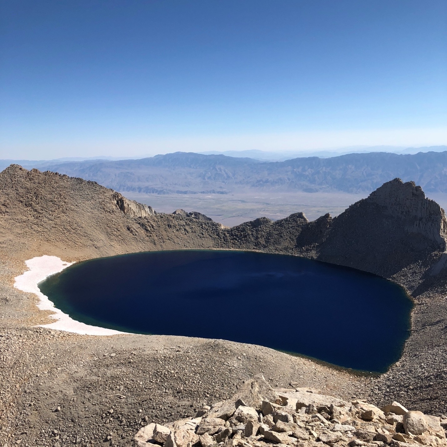
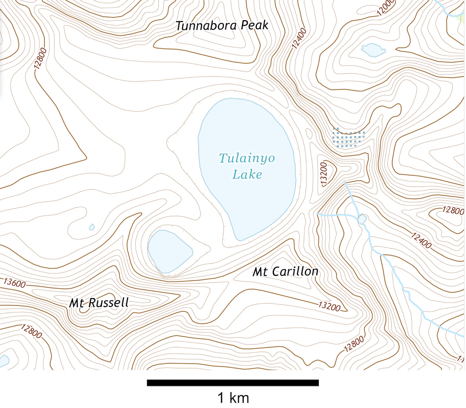
First, mark on the map where the photo of Tulainyo Lake was taken.
Where are the lowest and highest elevations in this map? ____________________
Next, look at the stream in the southeastern side of the map. What happens to contour lines when they cross a stream? Your instructor may also provide you with block models to illustrate this rule.
Tulainyo Lake and an unnamed lake in this map have little hatch marks around them. What do these mean?
Critical thinking: The contour interval is 100 m (328 ft). Do you think this is adequate to show the topography in this region (look at a photo of the area). What contour interval would you prefer and why?
Critical thinking: Normally, you wouldn’t see contour cross or meet on a topographic map. Can you think of any scenarios where contour lines would cross and/or meet?
Build your own contour map. Use the elevation data to make your own contour map from the data in Figure 2.13. The contour interval will be 10 m. The zero-contour interval is at sea level; so, you don’t need to draw that one! You may have to interpolate and extrapolate the data as there are very few data points that are 10 m intervals. Remember how the contour intervals should look around the small streams and rivers. Draw your contour lines so that they are continuous: they will either continue to the edge of the map or form an enclosed circle.

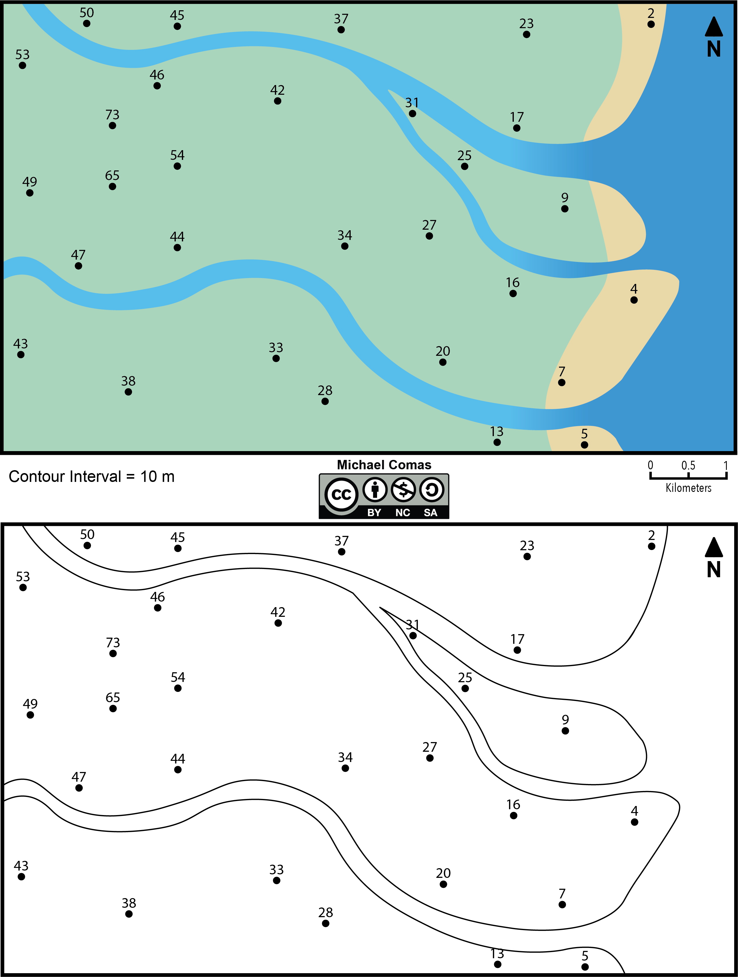
Figure 2.13 – Upper: Map for contouring in color; Lower: Same map but black and white. Image credit: Michael Comas, CC BY-NC-SA.

So, if you are lost, how are you going to find yourself on a map as you won’t always be able to rely on the GPS position in your phone for reliable location data. First, keep the map facing the right direction using the compass rose. Then, look for big landmarks like mountains or rivers to match with the map. In the wilderness, seek out prominent natural features to triangulate your position. Once you’ve identified your location, orient your map so that North is at the top and continue your hike.

Exercise 2.8 – Finding Yourself on a Map

Now that you have a good understanding of some map basics, let’s get some practice finding specific locations on a map.

1. Figure 2.14 is a photograph from somewhere around Mt. St. Helen’s in Washington State. Figure 2.15 is a satellite imagery map of the Mt. St. Helen’s area. Use clues from the photograph to locate the position of the photographer and mark it on the map.
  
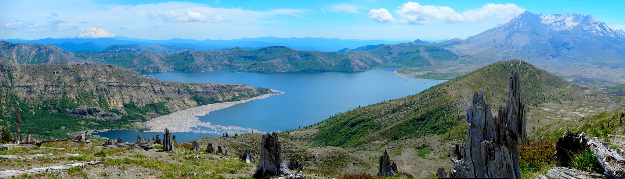
  Figure 2.14 – Photograph taken from the Mt. St. Helen’s region. Image credit: Alejandro Rodriguez, CC BY.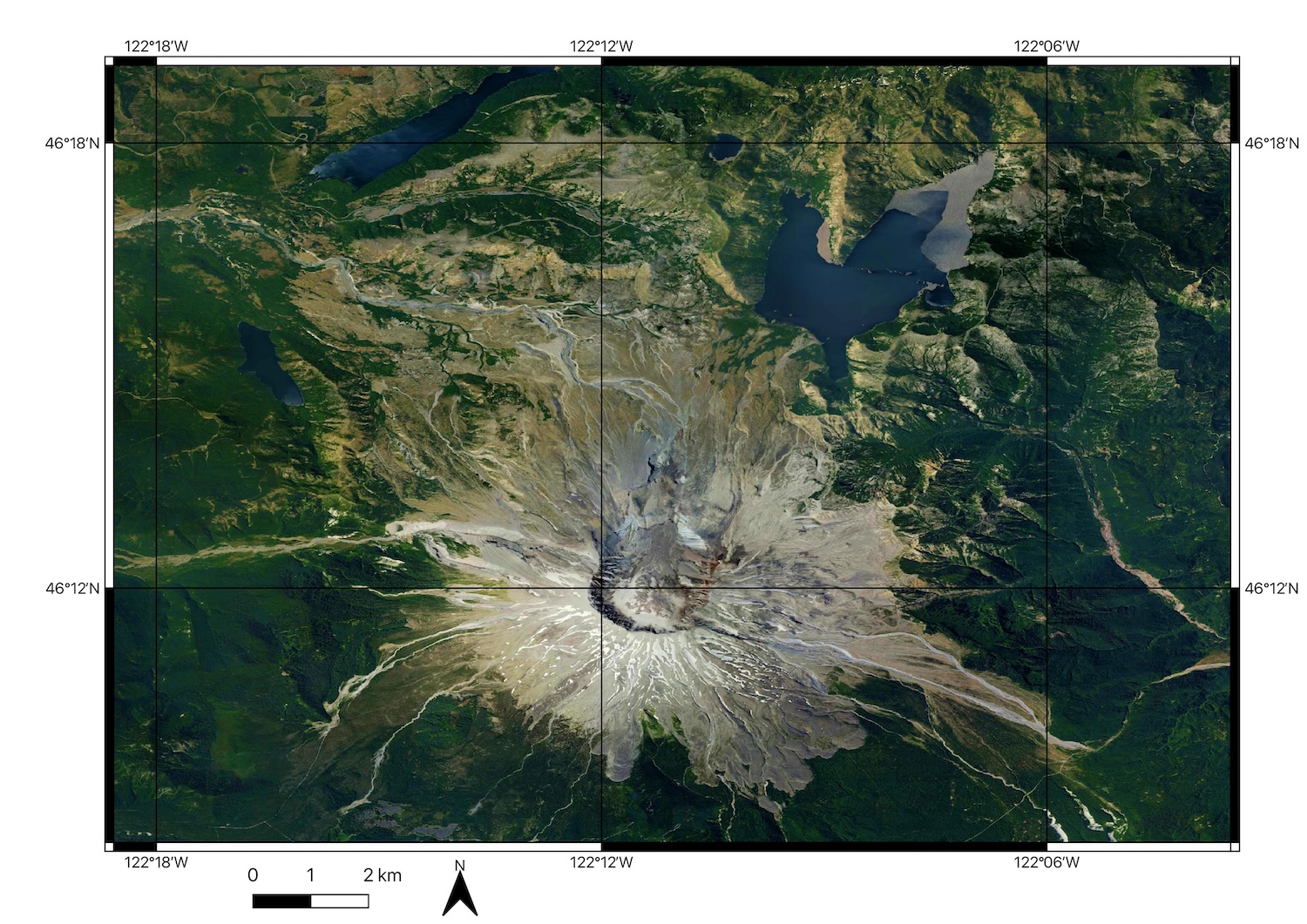
  
  Figure 2.15 – Satellite imagery of the Mt. St. Helen’s region. Image credit: from Bing Maps; TomTom, Earthstar Geographics.
2. Figure 2.16 is from a photograph from Grand Teton National Park in Wyoming, and Figure 2.17 is a topographic map of the surrounding location. Determine the location the photo was taken from and mark it on the map.
  
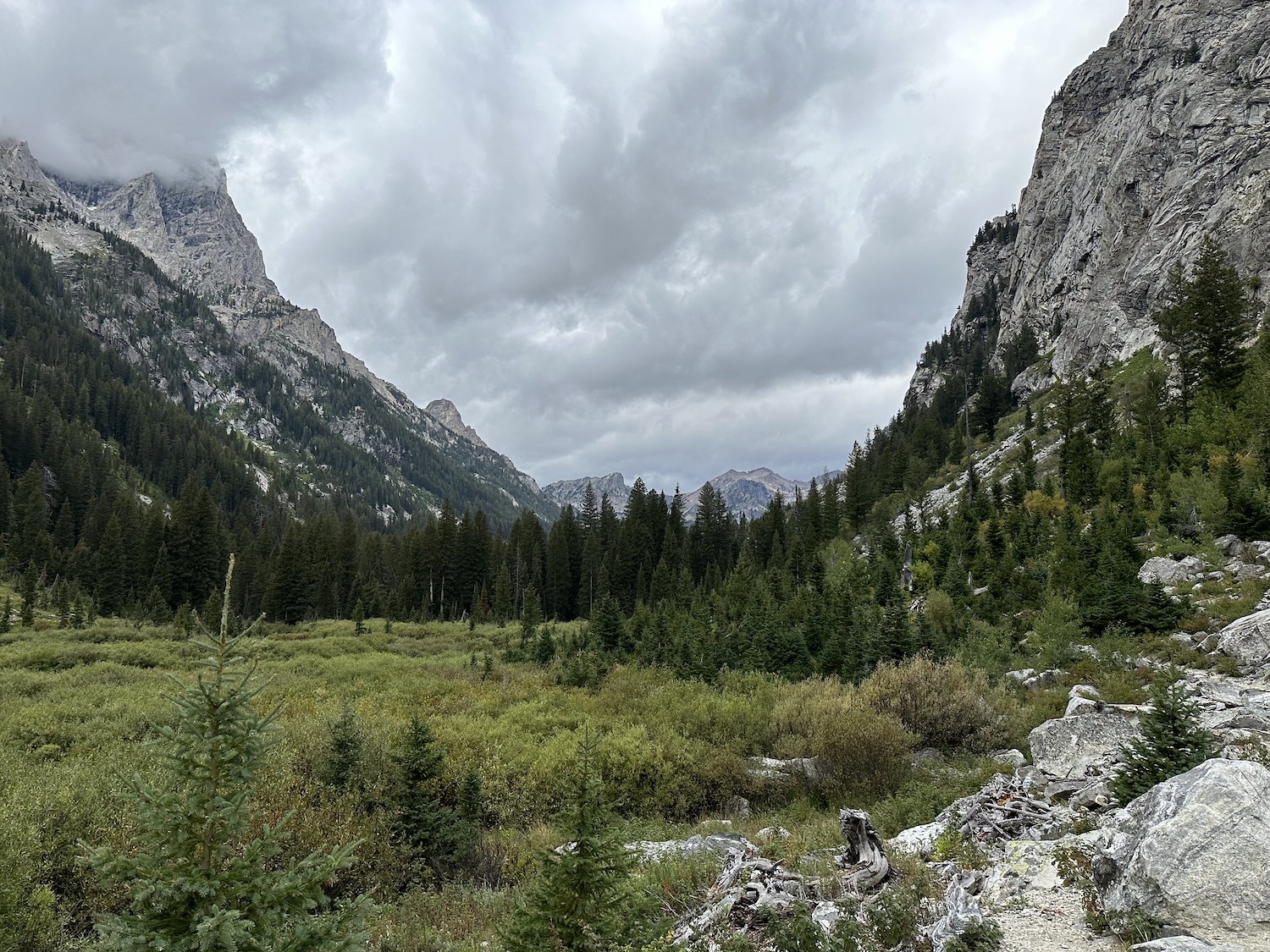
  Figure 2.16 – Photograph from a hiking trail in Grand Teton National Park, Wyoming. Image credit: Michael Sprague, CC BY-SA.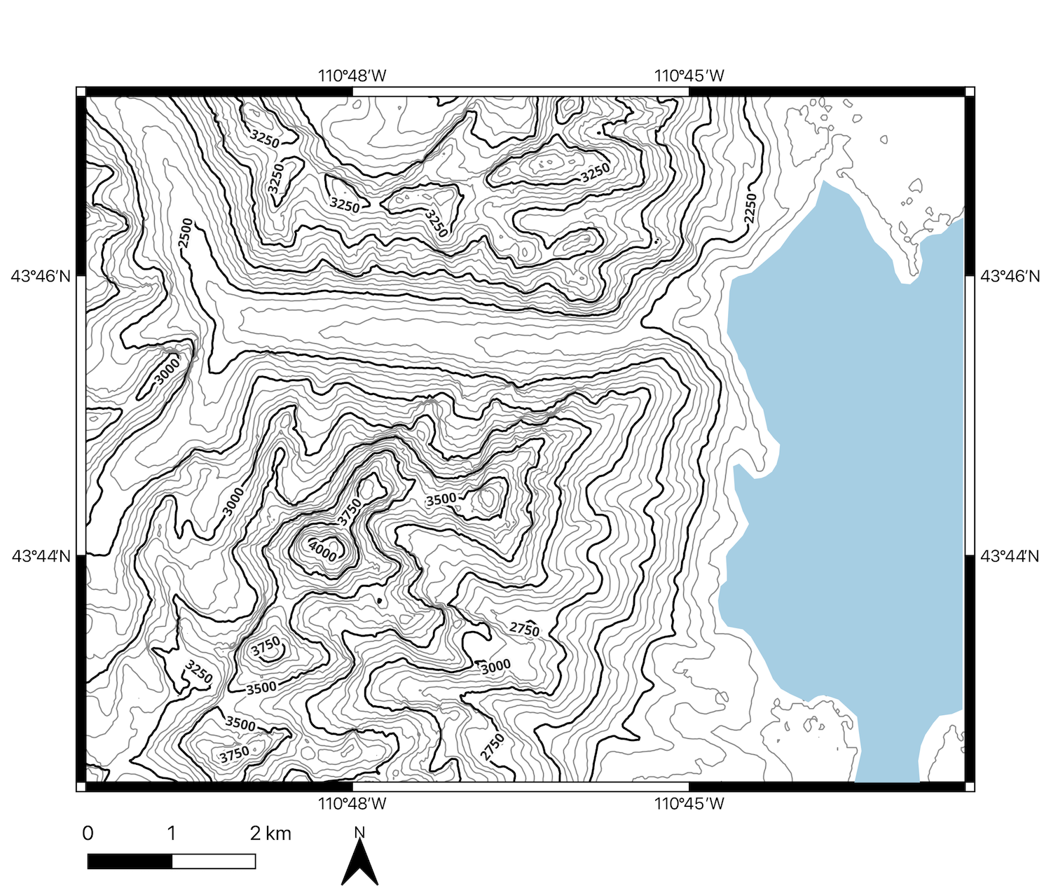
  
  Figure 2.167- Topographic map for part of the Grand Teton National Park area. Image credit: Daniel Hauptvogel, CC BY-NC-SA.

Most of now use our cell phones with built in GPS, maps and apps to help us decide where to go. Even with these, you hear stories of people blindly following these and ending up on roads that dead end or are closed due to weather. Or you may go someplace without cell signal to be able to use your map app. So, knowing how to read a topographic map, is a useful skill for these and other situations.

Exercise 2.9 – Navigating with a Topographic Map

You and your friends are planning a hiking trip through Enchanted Rock State Natural Area (Figure 2.18 and 2.19). All the camping spots near the main parking lot are reserved. So, instead your group wants to camp in a backcountry at either Moss Lake or Walnut Springs. Some of your friends also want to go rock climbing.

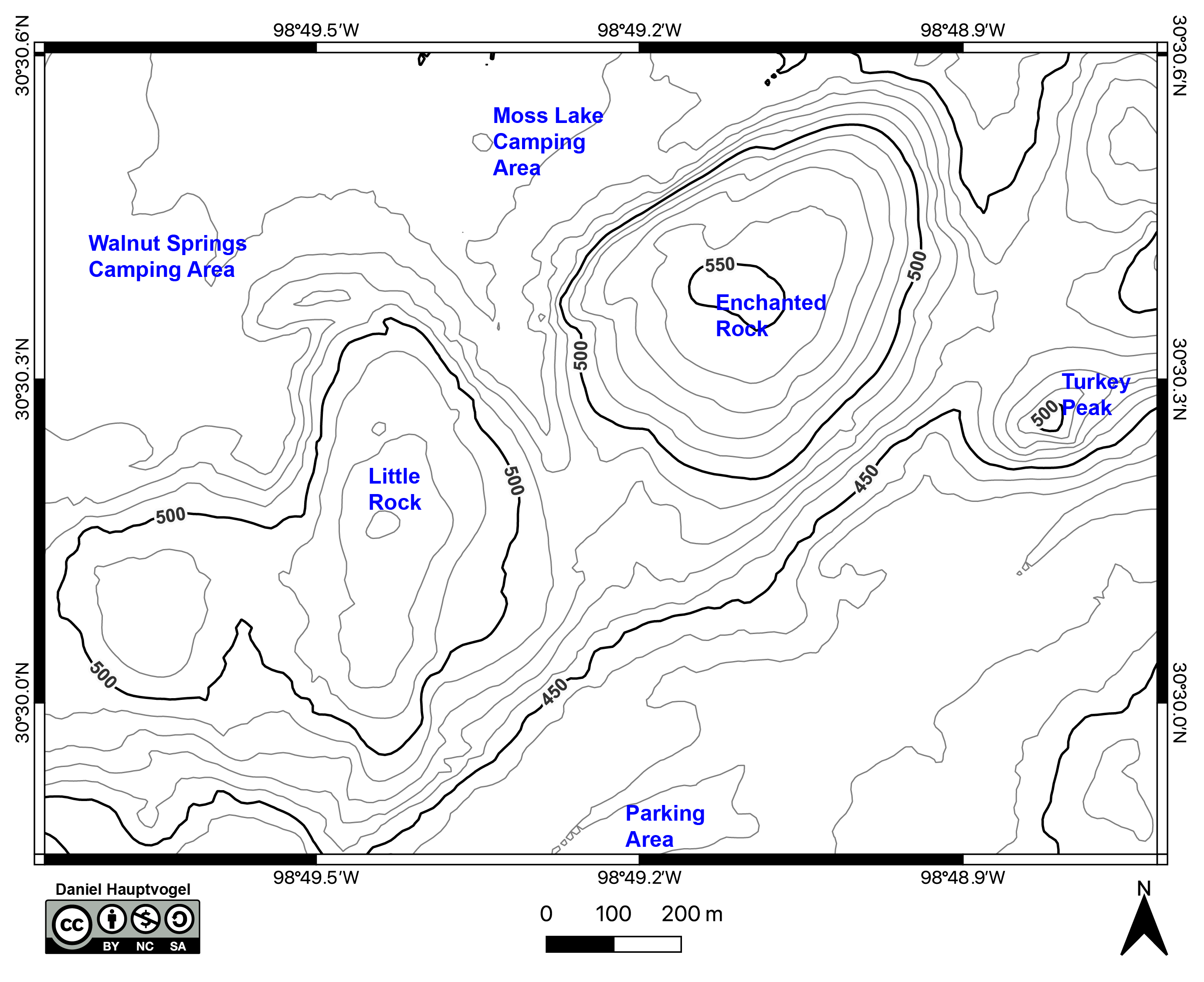
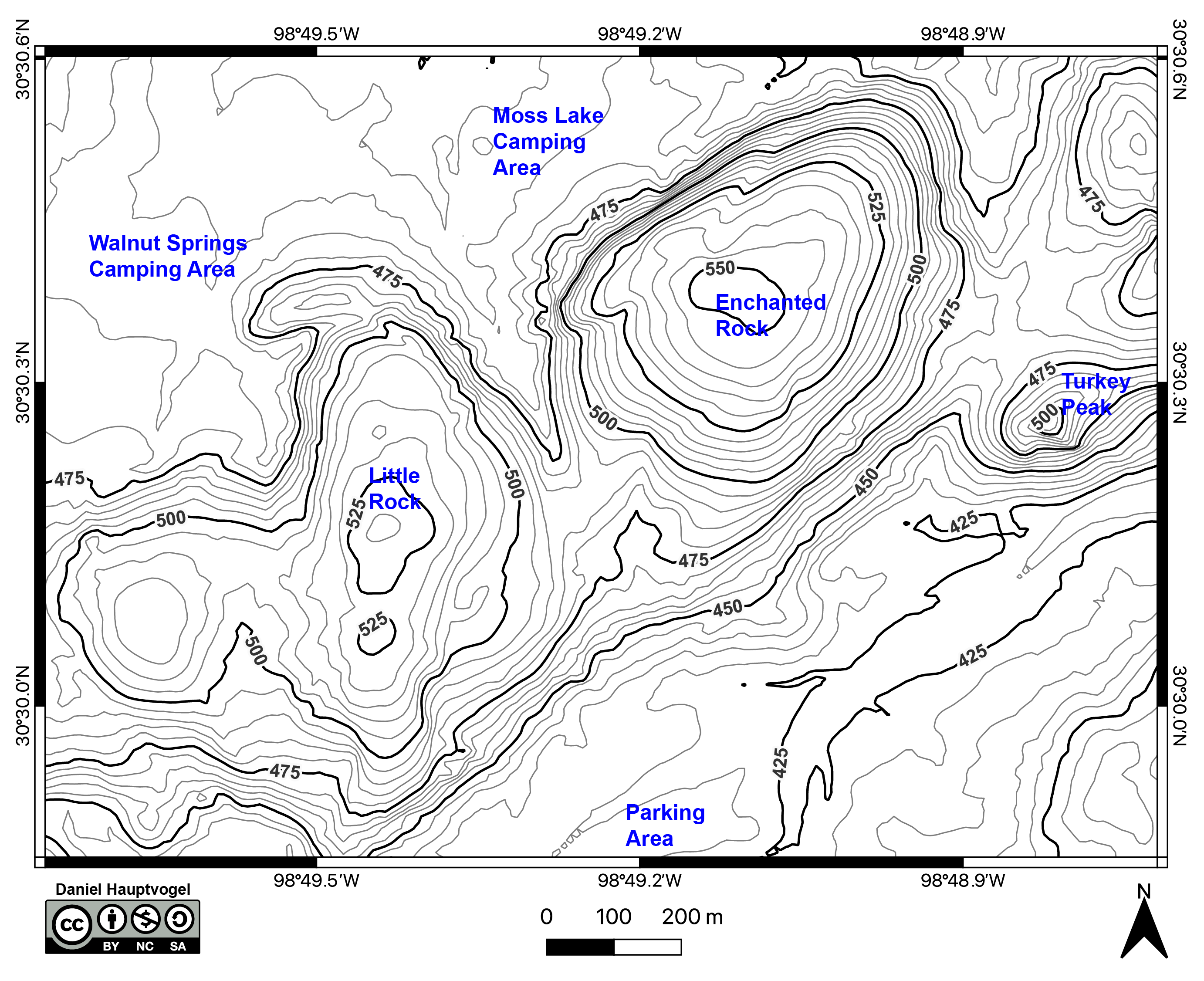
Contour map of Enchanted Rock State Natural Area, TX — Figure 2.18 – Topographic map of Enchanted Rock State Natural Area with 10 m contour intervals. Also shown are main parking lot and two backcountry campgrounds. Image credit: Daniel Hauptvogel CC BY-NC-SA, data from USGS.

One of the choices, a cartographer (map maker) has to make is the contour interval. Figures 2.18 and 2.19 are the same map with different contour intervals at either 10 or 5 m. Chose one of these for answering the following questions. Why did you chose this map?
Estimate the elevation for the following points:
1. Enchanted Rock: ____________________
2. Little Rock: ____________________
3. Parking Lot: ____________________
There are two possible back country camp grounds at either Moss Lake or Walnut Springs. Chose one for your group. Draw two possible routes to this back country camping area from the parking lot. What is the length for each route?
1. A: ____________________
2. B: ____________________
What is the elevation gain for each route:
1. A: ____________________
2. B: ____________________
Which trip route would you take? A or B? Explain your reasoning.
You and your friends decide to hike to the top of Enchanted Rock. Since the entire dome is just rock, you can go almost anywhere to get to the top. You want to take the path with the lowest slope because it will be easier. Draw the best path to take on Figure 2.18.
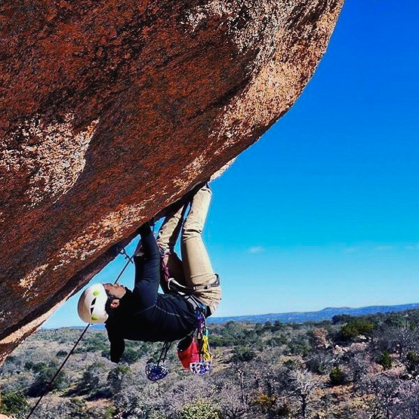
You and your friends want to go rock climbing (Figure 2.20). They think there are several possible places with very steep topography. Which place has the steepest topography? Circle it on either Figure 2.18 or 2.19.

Rock climbing at Enchanted Rock State Natural Area TX — Figure 2.20 – Rock climbing near Freshman Mountain at Enchanted Rock State Natural Area. Image credit: Caitlin McNulty CC, enhanced by Alex Maze.

2.3 Topographic Profiles

To get a sense of the landscape, geologists construct topographic profiles (Figure 2.21). One choice that profilers make is whether the vertical scale is the same or different from the horizontal scale. This decision is called vertical exaggeration (VE) and is used to emphasize vertical features. It makes terrain features or objects appear larger, increasing their visibility. VE can be useful in visualizations of terrain where the horizontal scale is significantly greater than the vertical scale. For example, if you wanted to show subtle topographic features in a relatively flat area, then you might expand the VE. This is often abbreviated as VE = 1:1 or VE = 5:1 meaning that the horizontal and vertical scale are the same or that the vertical scale is five times larger than the horizontal scale

To do make a profile, use these five steps:

Place a strip of paper along the line of the profile you are making (W-E) and label the starting and ending points (Figure 2.21).
Mark the paper where it comes into contact with any contour lines and label each mark with the corresponding elevation.
Choose your vertical scale and prepare a sheet of graph paper by labeling the vertical axis according to the scale you have chosen. It is typically best to choose a range of elevations that encompass your profile elevations (for example, if the Volcano’s elevations ranged from 223-339 meters, it may be best to choose a scale from 200-350 meters).
Place your strip of paper with the labeled marks (from Step 2) at the bottom of the vertical scale and use the elevation data to plot points on your graph.
Trace the points from one side of the profile to the other.

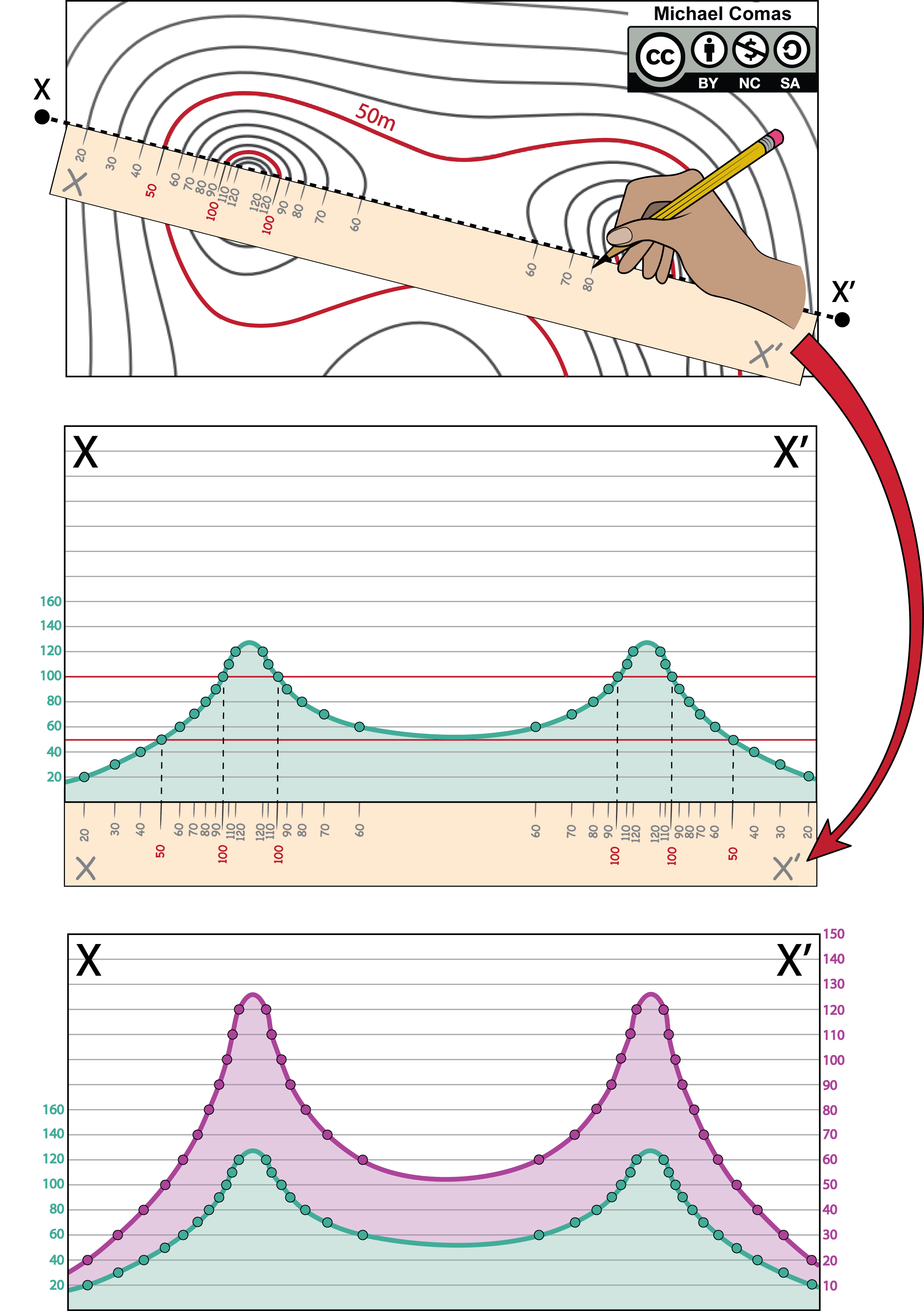
Figure 2.21 – How to construct a topographic profile using the steps outlined in the text. The purple line on the bottom figure shows vertical exxageration as the vertical scale is twice the horizontal scale or VE = 2:1. Image credit: Michael Comas, CC BY-NC-SA.

Exercise 2.10 – Constructing a Topographic Profile

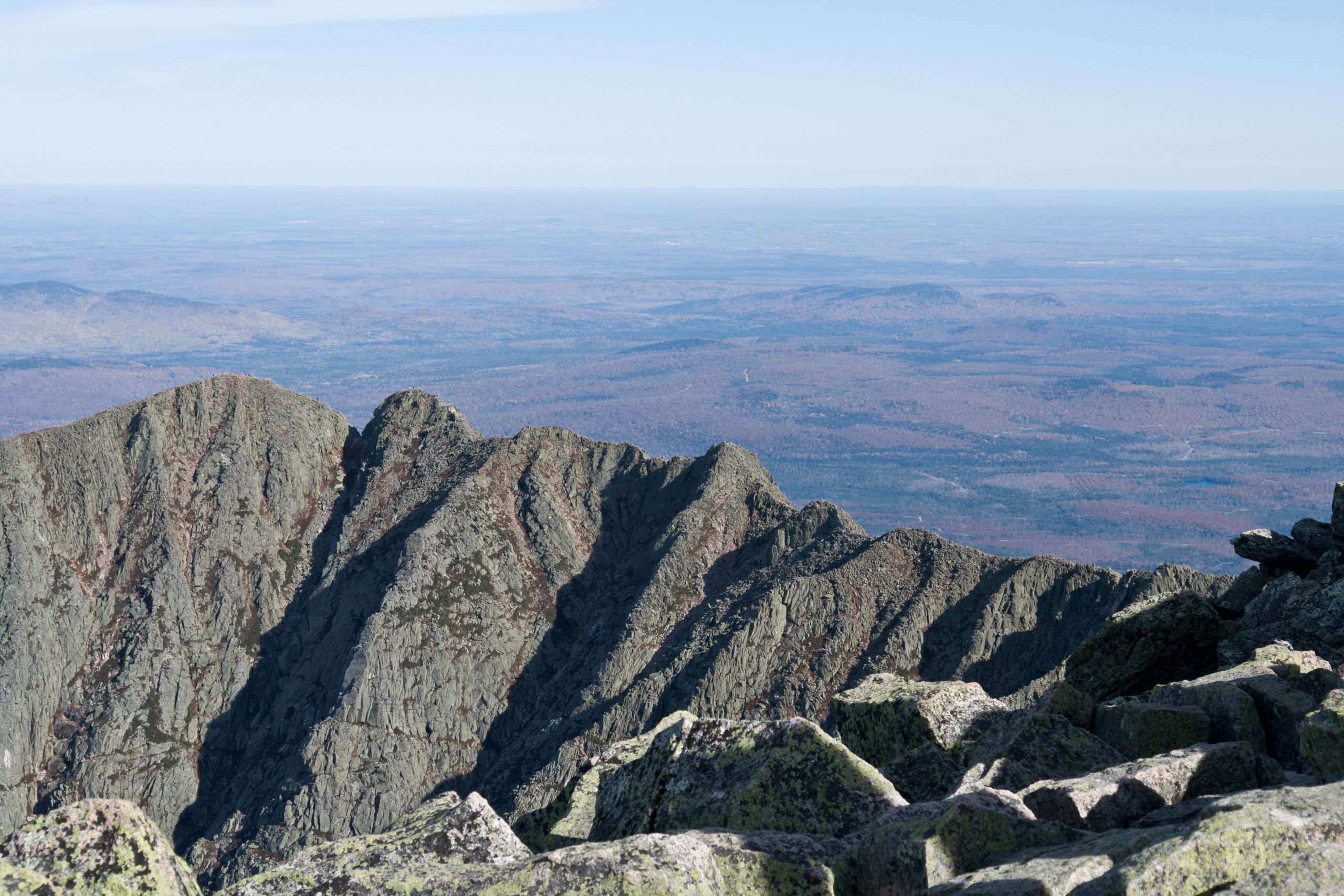
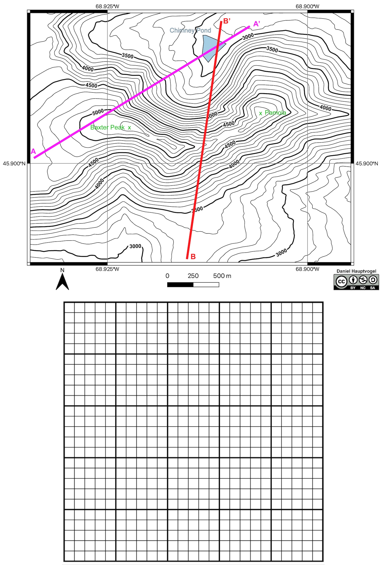
Mount Katahdin is composed of five peaks; two of these are shown in Figures 2.22 and 2.23. One of these, Baxter Peak, is the northern end of the Appalachian Mountain Trail which extends from Georgia to Maine. Construction of this 3,525 km (2,190 mile) long public footpath was started in 1921 and finished in 1937. Mount Katahdin is a large igneous sill or laccolith intruded during the Acadian orogeny at ~407 Ma. This supervolcano also erupted the 407 Ma Traveler’s rhyolite. More recently, Mount Katahdin was carved by glaciers first by the Laurentide Ice Sheet and more recently by valley glaciers at ~15,000 years ago.

Make a topographic profile for Figure 2.23 using either line A-A’ or B-B’.
What is your vertical exaggeration (VE)? Why did you choose this vertical scale?
Using your profile, describe the difference between the northern and southern ends of your profile.
Can you identify which side of Mount Katahdin was carved out by a valley glacier. This type of landscape is called a cirque. Explain your answer.
Critical Thinking: If you hike between Baxter and Pamola peaks, you will traverse a feature called the Knife’s Edge which in some spots is only ~1.2 m (4′) wide with each side dropping off 610 m (2000′). Does your profile show this precipitous drop? How would you let a hiker know about this feature in your profile?