
Chapter 10: Deformation and Structures
Brittle and Ductile
Learning Objectives
The goals of this chapter are to:
- Understand geologic deformation and structures
- Interpret brittle and ductile structures
- Evaluate three dimensions of deformation
10.1 Deformation
The deformation of rock layers can make interpreting the geologic history of those layers more difficult. However, it can also tell us about the tectonic processes that may have occurred in the region. For these reasons, geologists must understand how deformation of rock layers occurs and how to deconstruct the often confusing structures that result from deformation. Then, the original position of the rock layers can be determined. Remember that these tectonic processes can occur on vastly different spatial-temporal scales and can vary based on the type and thickness of rocks that are being deformed, so no two faults or folds will be exactly alike.
Exercise 10.1 – Observing Deformation
Your instructor has placed a block model on your table.
- Create sketches of the block model from at least two different viewpoints.
Table 10.1 – Block sketches Sketch 1: Sketch 2: - Describe what you think is significant about your block model.
To identify different types of deformation, you first need to be able to recognize bedding and foliation planes (layers). Look for distinct changes in color, breaks between layers or foliation, changes in lithology, etc. When you look at an outcrop, first try to identify the bedding or foliation. This may be horizontal or tilted. Folded, tilted, faulted bedding and foliation planes are useful markers that allow you to investigate deformation structures in rocks. They can be continuous and followed for long distances or shorter if the depositional environment has local changes.
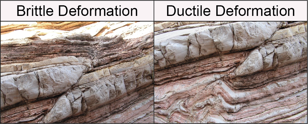
You can identify deformational features by tracing these bedding and foliation planes. Only two dimensions are often visible, and you need to infer the third dimension. So, look at the outcrop and note if the bedding/foliation planes are straight or curved. If they are curved, the rocks deformed by bending or flowing (ductile) and are folded. If they are straight, then you are looking at brittle deformation. What controls brittle (breaking) versus ductile (bending) are complex interactions between temperature and rock types. Remember how deep you observed earthquakes occurring? Earthquakes are brittle deformation and occur at shallow depths and low temperatures. As temperature increases, the rocks switch to ductile deformation, and there are no more earthquakes.
Figure 10.1 shows how rock type controls whether the rocks bend or break. The shales bend, whereas the sandstone breaks. Are the bedding planes discontinuous across a break in the rocks? If they are discontinuous, this typically indicates a brittle fault. In this case, follow a few bedding planes, and if they are continuous, you are seeing folds and ductile deformation.
10.2 Ductile Deformation
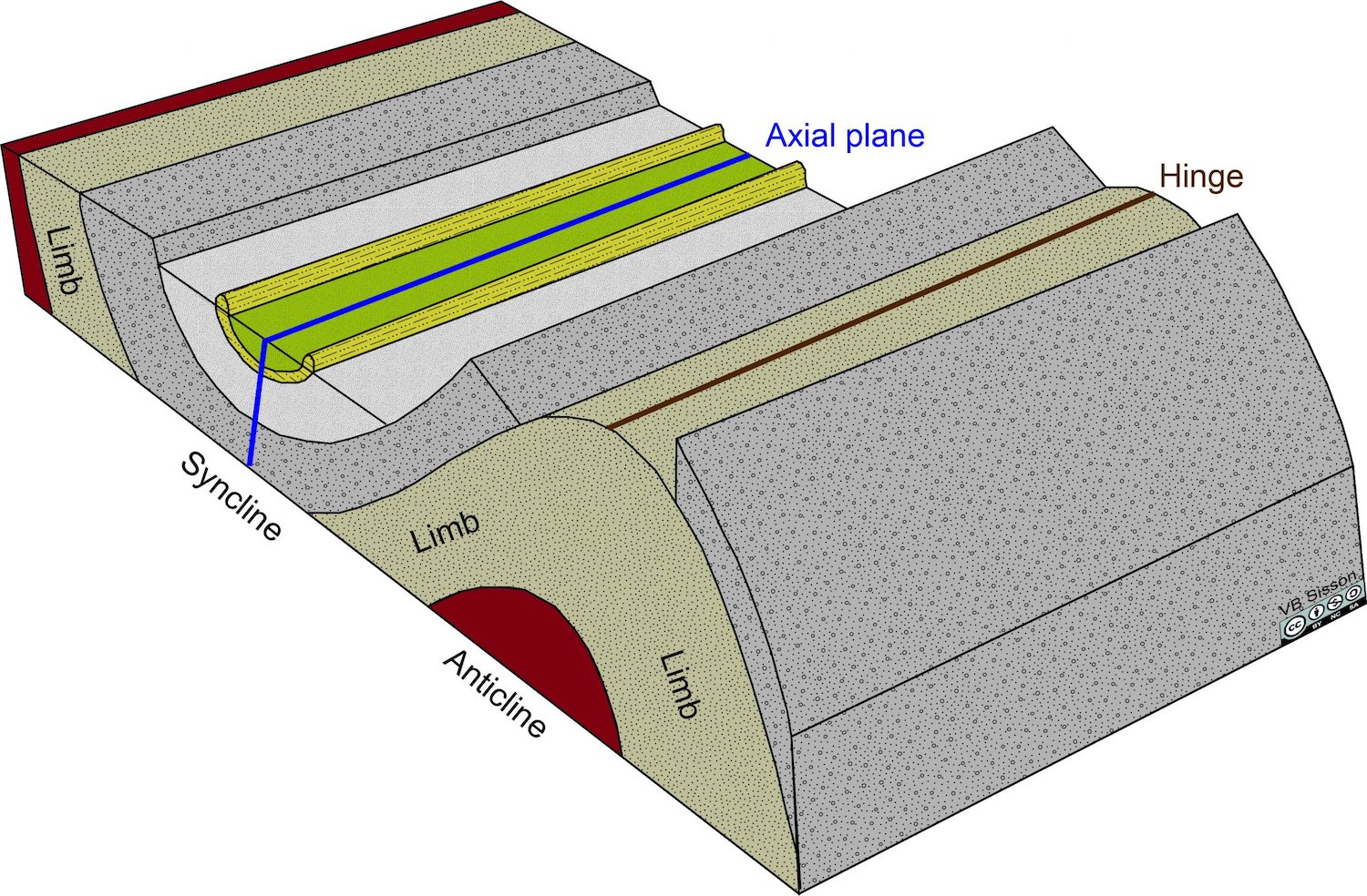
Folds form when layers or beds are bent or folded due to convergent plate tectonics. They can be rounded or angular. The plane that marks the center of the fold is called the axial plane. The line that marks where the axial plane intersects the surface of Earth is called the hinge line. The areas on either side of the curved hinge zone stick out like arms or legs and are appropriately called limbs. There are often several folds connected (see Figure 10.2). If the bedding planes tilt down from the axial plane, this is an anticline (easy to remember since it sort of looks like an A). However, if the bedding planes tilt toward the axial plane, this is a syncline (Figure 10.1). Folds are common in convergent plate boundaries.
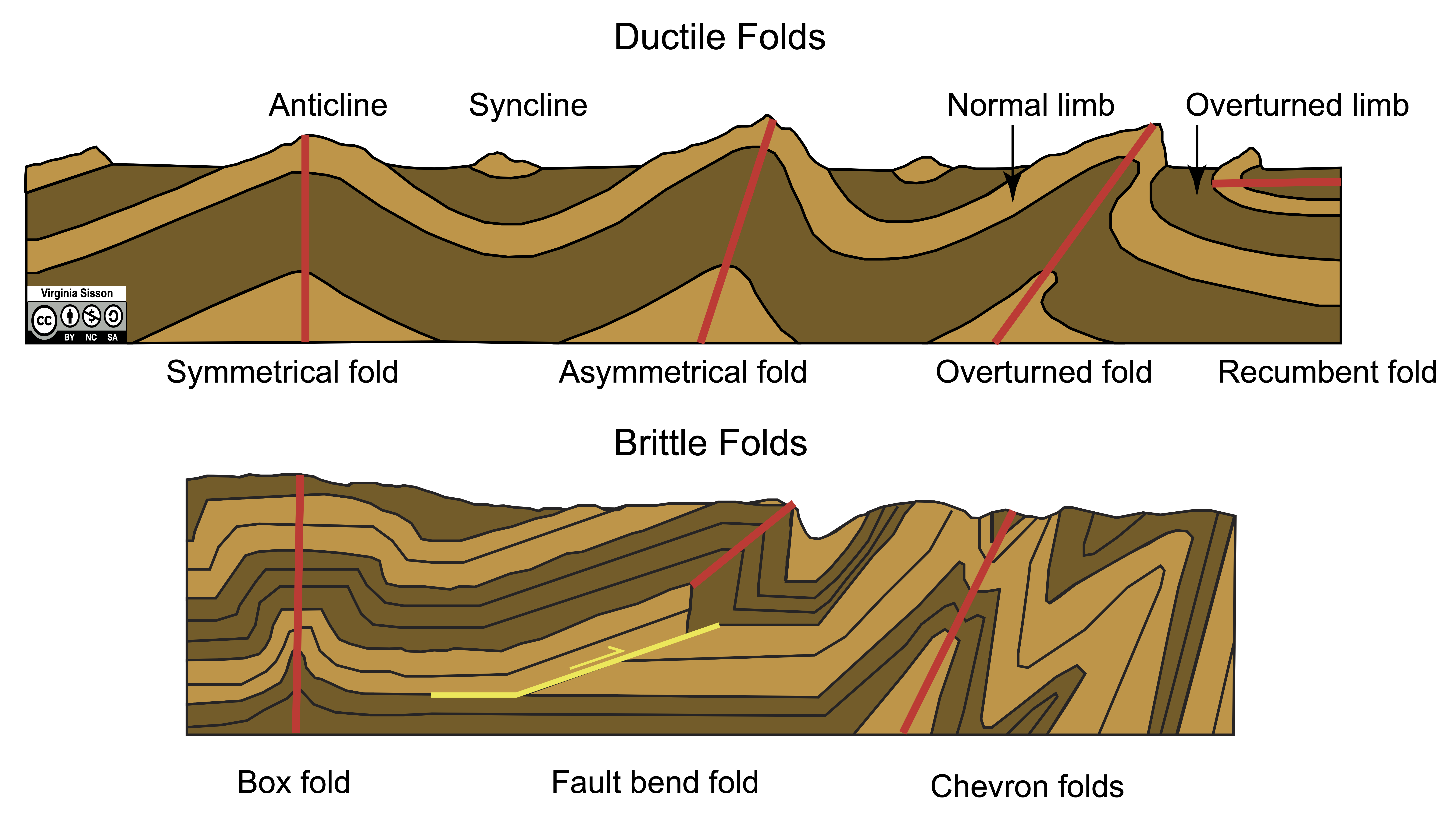
Folds vary in size and shape. Some cover hundreds of kilometers in width, and others measure a few centimeters or less. Folds are generally classified according to the orientation of their axial plane, which can be vertical, horizontal, or inclined at any intermediate angle. In addition, the angle between the axial plane and the fold limbs is important for classifying folds. The angle of the axial plane relative to horizontal is called plunge. So, in addition to the folds shown 10.2, there are a variety of other folds shown in Figure 10.3. These include ductile folds:
- Symmetrical – vertical axial plane with the same dip for both fold limbs
- Asymmetrical – axial plane is tilted with a shallower dip on the left fold limb compared to the right fold limb
- Overturned – axial plane is tilted and the left limb has a shallow dip whereas the right limb with the stratigraphy overturned (upside down)
- Recumbent – horizontal axial plane with the same dip for both fold limbs
and brittle folds:
- Box – rectangular fold in which the fold limbs are right angles. This fold has three limbs
- Fault-bend – tilted axial plane and angular fold limbs. These form over thrust faults (see next exercise)
- Chevron – tilted to vertical axial planes with straight limbs that abruptly bend at one point at their hinge zone.
Exercise 10.2 – Identifying Folds
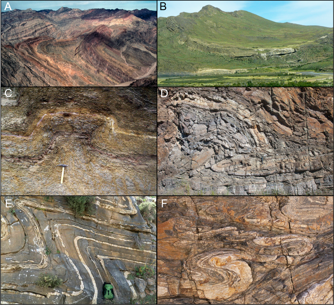
Folds can be both brittle (bent) and ductile (rounded) features. Figure 10.4 shows six photos of folds. These start as large mountain scale folds (A and B) and get smaller and more complicated (C to F). There are geology rock hammers for scale in images C and D.
- For each photo, identify the type of fold shown and the direction of stress needed to create it. There is more than one fold in E and F.
- Sketch the axial plane(s).
- Indicate the age of the sedimentary units with “o” for oldest and “y” for youngest.
- Describe the characteristics of the folds by filling out Table 10.2. Some characteristics include what is the dip of the axial plane and are the dips of the layers similar on both sides of the fold, symmetry of fold (dip of each limb relative to axial plane), type of fold (anticline, syncline, inclined, recumbent, box, fault bend, etc.). Since folds form in convergent tectonic settings, you don’t need to determine the tectonic setting for these features
| Photo # | Brittle or Ductile | Angle of Axial Plane | Axial Plane Curvature | Fold Symmetry | Type of Fold |
|
A
|
|||||
|
B
|
|||||
|
C
|
|||||
|
D
|
|||||
|
E
|
|||||
|
F
|
10.3 Brittle Deformation
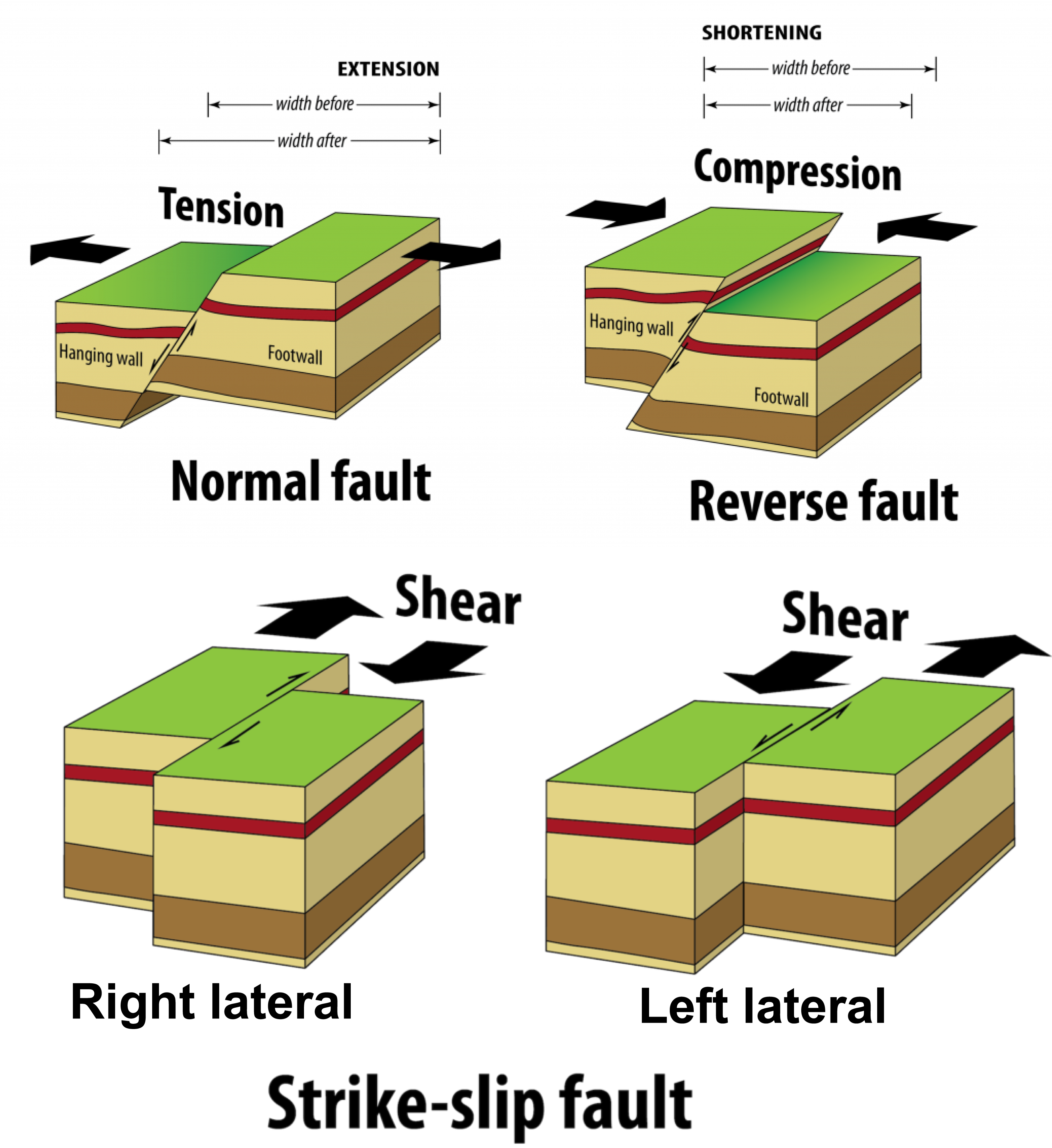
Let’s go over faults. First, ask yourself if you are looking at the Earth’s surface or a slice (cliff or outcrop along a road) through the Earth. Once you’ve done that, you will know if you are looking at either vertical (up and down) or horizontal (side to side) motion.
Vertical motion is called dip-slip. If the motion is mostly down, then this is a normal fault. If the motion is up, it is a reverse or thrust fault. The difficulty is deciding if the motion is up or down. To help with this, imagine standing with the fault above your head. Your feet are on a layer that doesn’t move. Some call this the footwall. The rocks above your head are called the hanging wall, as they might come crashing down on you. Then, do you have to look up or down to find this same layer on the other side of the fault (Figure 10.5)? The difference between a thrust and reverse fault is how steep the fault is. If the fault is shallow, this is a thrust fault. If it is steep, this is a reverse fault. Reverse faults are common in divergent tectonic settings, whereas thrust and reverse faults are common in convergent tectonic settings.
Horizontal motion is called strike-slip or transform; these are common in transform plate boundaries. If you have a vertical section through a strike-slip fault, one side will move toward you and the other away. From the top view, see if the features moved to the right or left. Imagine you’re on one side of the fault, standing on an object cut in half by the fault. Then, look across the fault and see if the other half of the object has moved to the left or right. It doesn’t matter which side of the fault you are on (see Figure 10.4).
Exercise 10.3 – Identifying Faults
Figure 10.6 shows six photos of faults. Describe the characteristics of these faults by answering the following questions and filling out Table 10.3.Determine which view you are looking at. Remember that images can either be taken from above a feature showing a map view or from the side which is a cross-section view
- On each photo, draw a line for the fault.
- Identify the type of fault shown.
- If a fault is a dip-slip fault, identify the hanging wall and footwall on the photo and the approximate angle of the fault from the ground level.
- If it is a strike-slip fault, identify if it is left-lateral or right-lateral.
- Give the tectonic setting needed to create it.
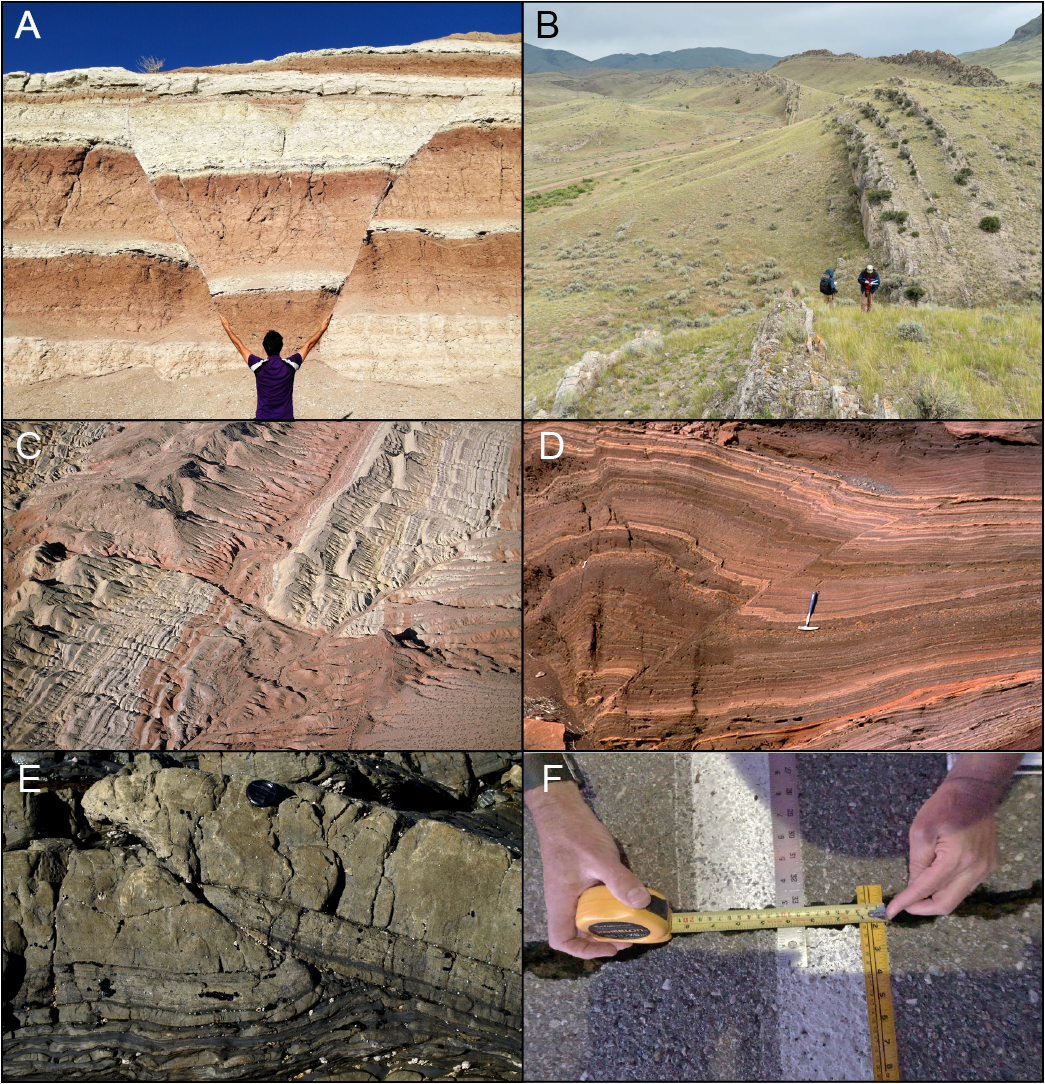
Figure 10.6 – Six images of brittle deformation. Images are from: A. Zanjan-Tabriz highway, Iran; B. Southwestern MT, C: Death Valley CA (note road cross-cutting the image); D. southeastern OR; D. Cape Liptrap, Victoria, Australia; D. Highway 176 near Ridgecrest CA. Image credit: A. Mohammad Goudarzi CC BY; B-D Marli Miller CC BY-NC-SA. E. Roberto Weinberg, used with permission, F. Kelly Blake, US Navy Public Domain.
| Photo # | View | Movement Direction | Fault Angle | Fault Type | Tectonic Setting |
|
A
|
|||||
|
B
|
|||||
|
C
|
|||||
|
D
|
|||||
|
E
|
|||||
|
F
|
10.4 Structures in Three Dimensions
Thinking about geology in three dimensions (3D) is difficult. If you practice, this is an ability that you can improve with time. If you can make 3D images of structures, you can figure out structures beneath you. In fact, some geologists say that the structure you see at the surface is similar to what is underneath. Click here for a 3D image of a fold. Is it the same from the top as well as the side?
Exercise 10.4 – Working in Three Dimensions
Figure 10.7 contains four block models of different types of deformation.
- Complete the remaining sides of the diagrams for Figure 10.7. Identify the type of deformation and its characteristics.
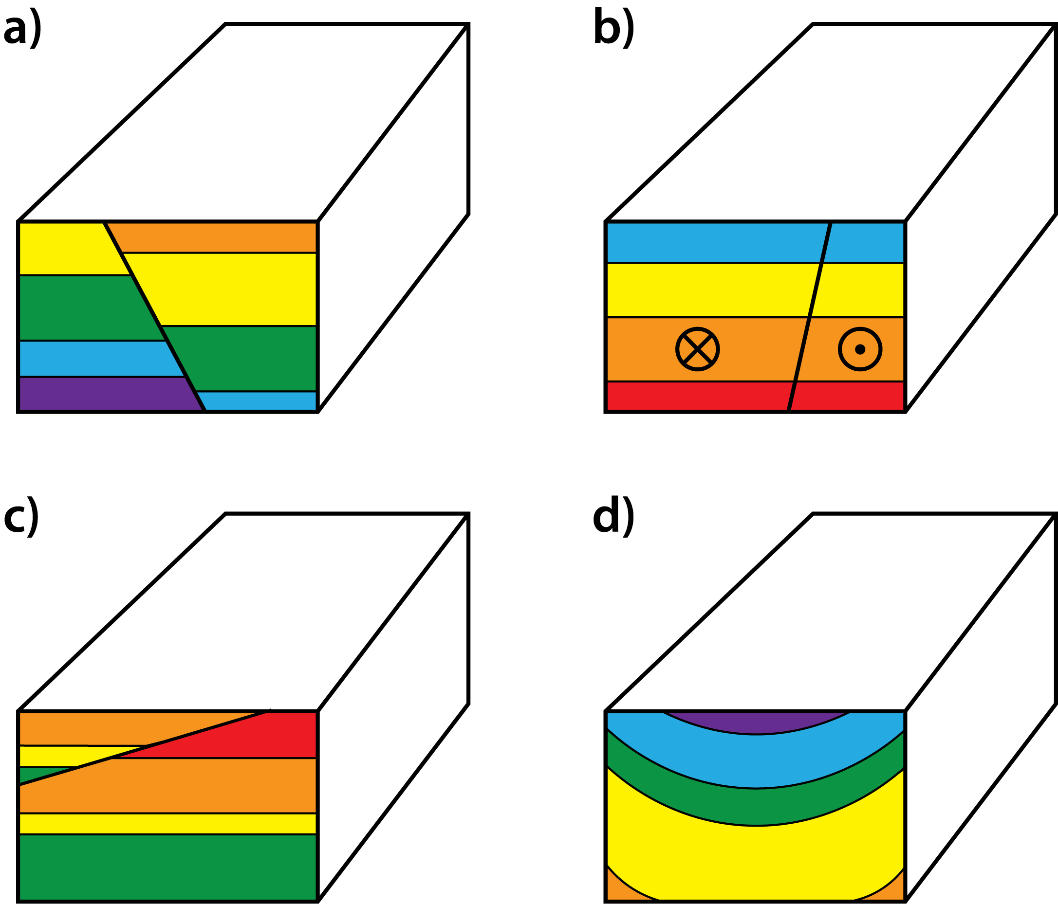
Figure 10.7 – Block models of deformation. In image b, the two circles show the direction of relative movement. The circle with a dot is the side moving towards you whereas the circle with an x is moving away from you. Image credit: Michael Comas CC BY-NC-SA. - Which block diagram(s) shows ductile deformation?
- For the blocks with brittle faults, use an arrow to show the relative movement for the hanging wall (side above the fault).
- Indicate on the map view of each block diagram the oldest and youngest sedimentary layers.
- Use what you have learned from completing the block diagrams above to construct a new block diagram of an anticline on Figure 10.8. The block should have four layers colored (from youngest to oldest): red, orange, blue, and purple.
Figure 10.8 – Blank block model. - Are the oldest or youngest sedimentary layers in the center of the fold.
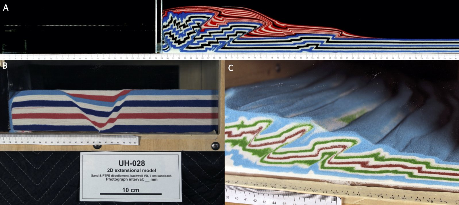
Since it is difficult to do experiments to deform rocks, geologists investigate deformation using analogs and modeling studies. An easy analog to use modeling clay. Start by making a few flat layers of different colors. Then use your hands as if they are two convergent plates and push on two sides of your clay layers. This will make a fold, either an anticline or syncline. Other geoscientists use sandbox models to replicate folds and faults (Figure 10.9). If you like programming in Python, you can try out GemPy to make your own 3D geologic models. However, for this class, we’ll use a simpler web-based program to make your own models of geologic structures.
Exercise 10.5 – Creating Your Own Geologic Structure
Head to Visible Geology to create your own geologic structure using the Geology Explorer tab. Click here if you need help using this website.
- Initially there are 3 layers of the same thickness. Start by adding 3 to 5 more layers. The first layer is the oldest (on the bottom). You can alter the rock name, height and color of the beds using the pen tool.
- Go to the Events tab to add a fold to your model using the Fold menu. You can rotate your model to see it in 3D. Use whatever orientation by changing the strike and dip of the fold axis. Be sure to click apply when finished. In Chapter 11, you will explore some of the other events and faults available in this website.
Answer the following questions.
- What is the color of the oldest bed? ____________________
- What is the color of the youngest bed? ____________________
- Is the fold in the center of your block a syncline or anticline? ____________________
- Are the limbs steeply or shallowly dipping? ____________________
- Where are the oldest beds in map view (view from the top)? ____________________
- Describe the differences between the side with the folds to the adjacent view to the right.
Often, geologists make geologic maps to show deformation features (more on that later). Now that satellites can provide images of the entire Earth’s surface, the first step in making a geologic map is to interpret satellite imagery. If you are going to work in an area covered by forests, another technique, LiDAR (Light Detection And Ranging) can be used to see below the canopy. For an example of folds shown with LiDAR, click here. Recently, geoscientists have turned to UAVs (unmanned aerial vehicles or drones) to get detailed imagery, creating either digital elevation models or hill shade maps of deformation features.
Geologists have borrowed the “Rule of Vs” to describe the geometry of mapped strata with respect to topography. The Rule also predicts the surface location of strata in areas of poor exposure. In the simplest case where a geologic feature is a vertical plane, the feature is a straight line. In contrast, if the feature is horizontal, the feature follows the contour lines. Keep in mind that the topographical expression of bedding represents erosional remnants of rock layers that once extended above the present surface; a lot of rock has been removed to produce the topography you see today.
Exercise 10.6 – Investigating Geologic Structures Using Google Earth
Use this Google Earth tour to explore some geologic structures.
- Stop 1 brings you to Canyonlands National Park in Utah. Describe the orientation of the sedimentary rocks.
- Are the sedimentary layers all the same thickness? Describe their characteristics.
- Has this area experienced any significant tectonic activity? Explain.
- Stop 2 brings you to an area near Mexican Hat, Utah. Look at the orientation of the rocks along the yellow line. What is the orientation of the sedimentary rocks on the western, central, and eastern parts of the line?
- Create a cross-section along that line. Your cross-section does not have to be to scale.
Table 10.4 – Cross-Section sketch Cross-Section: - What type of structures is this? ____________________
- Stop 3a brings you to the Spanish Peaks in Colorado. These are ancient batholiths of granitic rock that were exposed at the surface through uplift and erosion of overlying sedimentary rocks. Look at the 3b location. What is this feature? ____________________
- What is the orientation of this feature compared to the West Spanish Peak?
- Are there more features like this? Describe their relationship to the peak.
10.5 Structures on a Geologic Map
A geologic map is an important tool for many geologists. These maps show how rocks are distributed in an area, their relationships, and any geologic structures. In addition to the basic map information that you learned about in Chapter 11 (or 2), the age and rock types are described in the legend. As you know from the map you made of a volcano, the color of a unit may indicate its age. In addition, the pattern of the unit can indicate the rock type. There may also be information about faults and folds indicating fold axes and fault types. Other important geologic map data are the strike and dip of various features.
As in many other labs, one reason for studying folds and faults is that they are important for understanding and finding economic resources. For this reason, many geologists love anticlines. If an anticline has an impermeable layer such as a shale, it can act as a barrier to fluids moving through the Earth. Consequently, fluids will stop at this layer, trapping water, oil, and gas. Also, fluids can carry strategic elements such as gold. The Hill End anticline in Australia was mined and produced over 60 tons of gold!
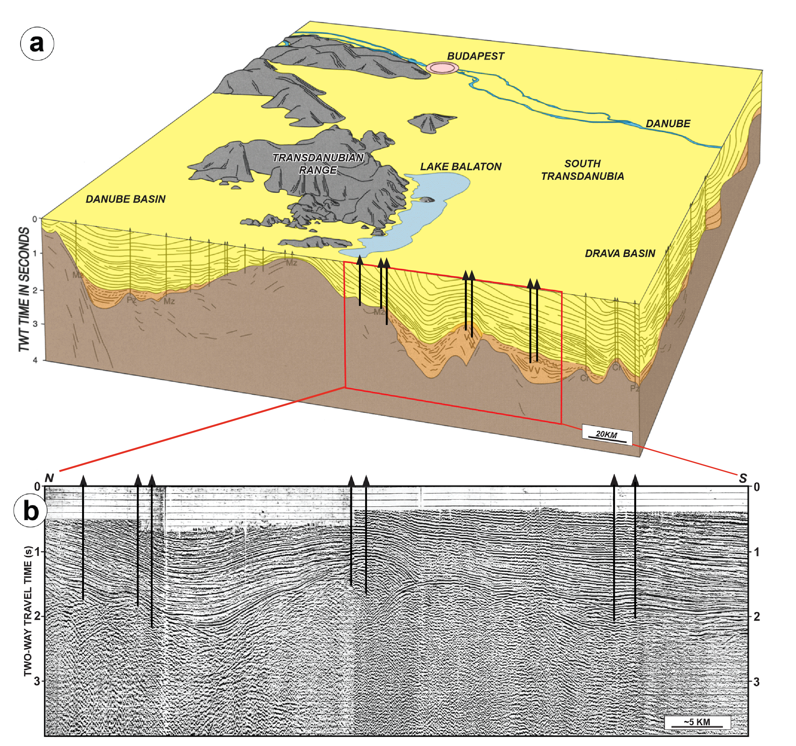
For the last 35 years, petroleum geologists have been using 3D imaging to understand geologic processes beneath the surface. Figure 10.10 shows two views of the subsurface below Hungary. On the right side of the figure, there are the sedimentary layers which are relatively flat. These formed in small rift basins. In contrast, in the center of part b, you can see an anticline with several oil wells. So, the anticline formed after rifting. This is not evident from the geology at the surface.
Exercise 10.7 – Exploring Geologic Structures Using a Geologic Map
First look at a satellite view of central Pennsylvania (Figure 10.11). Look at the patterns shown by areas with farms and areas with trees. At the top of the image, near the town of Shamokin, there are active coal mines. A locally famous geologic feature is the “Whaleback” exposed in an abandoned coal mine. If you want to explore this feature as a geology game, click on this link.
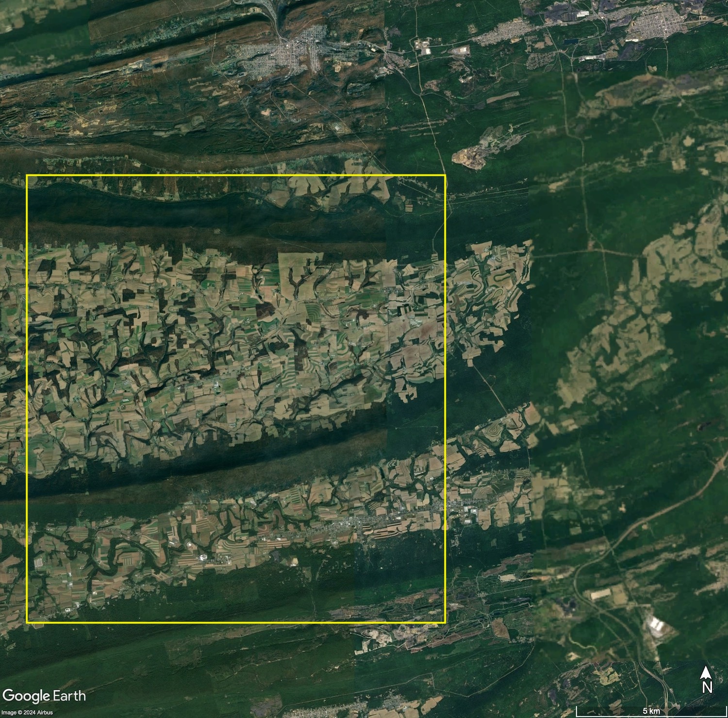
- Using this pattern, what type of deformation would you predict occurred in this area.
- Speculate why there are farms in some areas and tree in others.
- At the top of the satellite view is the town of Shamokin and at the bottom is the town of Valley View. Why do you think these towns are located in these areas?
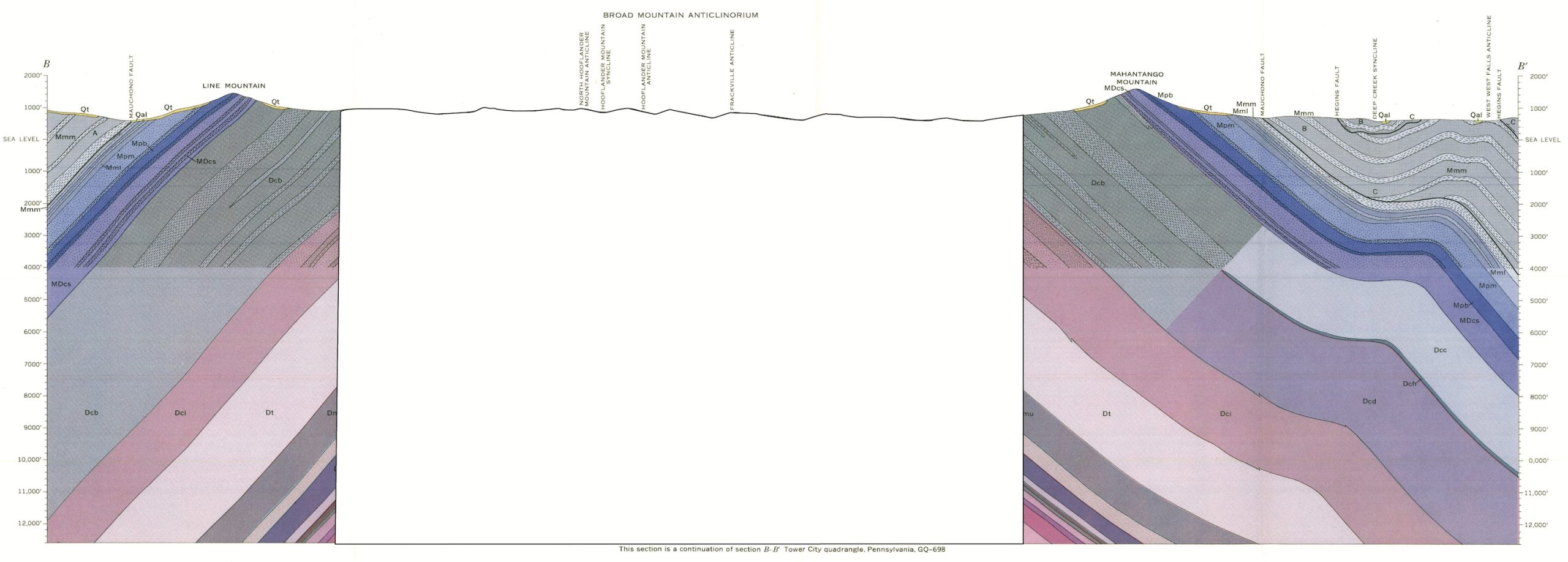
Now look at the geologic map shown in Figure 10.12. The important map components are labeled and outlined in boxes. Your instructor may give you a large version of this map to look at. There are many conventions about geologic maps; one that is useful for the next exercise is that rock units are presented in columns with the oldest sedimentary rocks on the bottom just like the law of superposition that you will learn about in the next chapter.
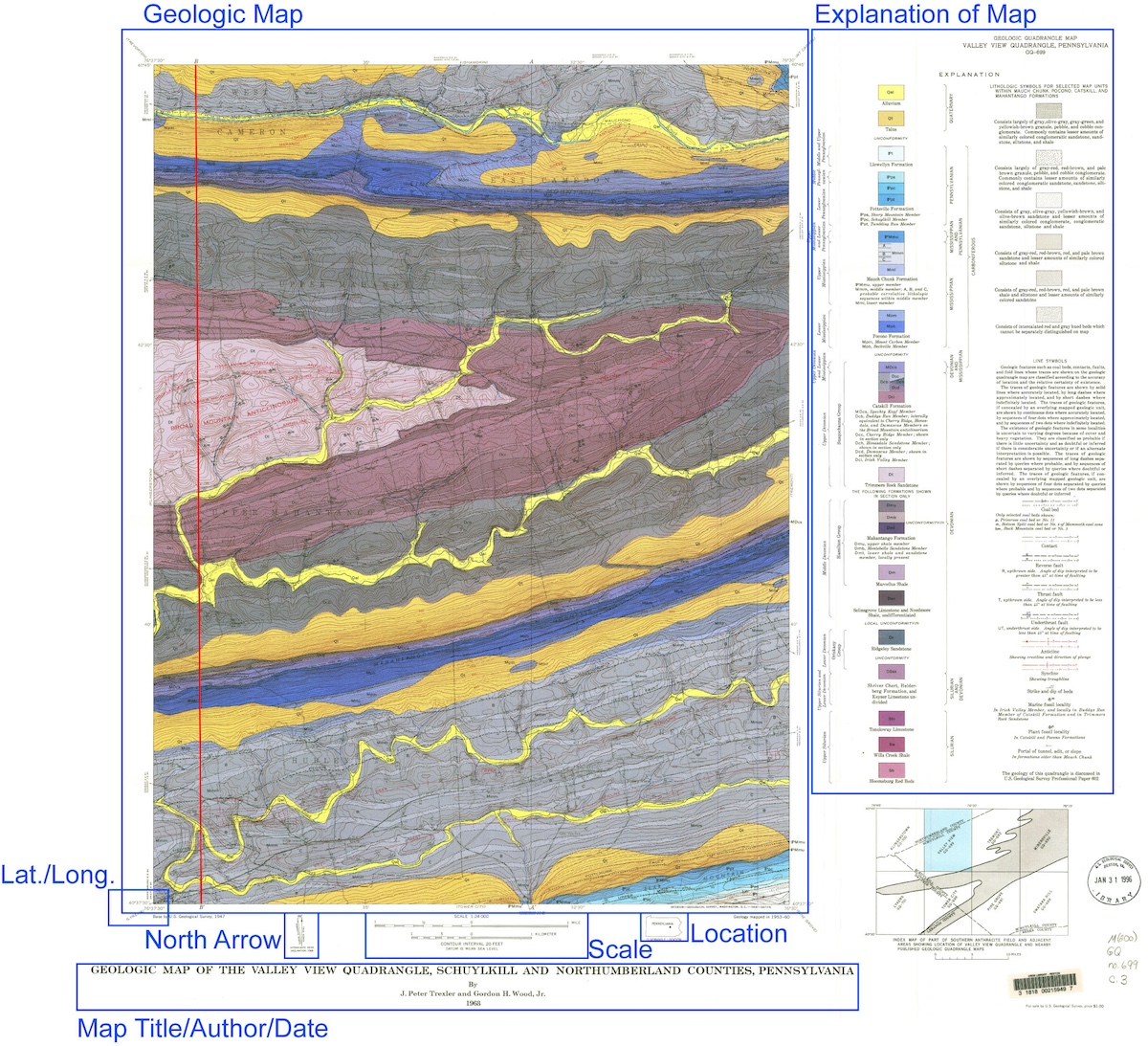
- Using the legend in Figure 10.12, what are the rock types in this area?
- Using the map and the legend, do the rocks become older or younger toward the center of the fold?
- Finish the cross-section in Figure 10.13.
- Notice that you can see a fold in both cross-section and map view. Why is this?
- Critical thinking: Pennsylvania has many oil and gas wells as well as coal mines. In fact, the first oil well ever drilled in the US was in Titusville PA to a depth of ~20 m (70 feet) in 1859. Do you think it would be good to drill a well for oil here? If so, how deep would you have to drill? Show your proposed location on Figure 10.12.
Additional Information
Exercise Contributions
Virginia Sisson, Daniel Hauptvogel, and Michael Comas
References
Tari, G., D. Arbouille, Z. Schléder, and T. Tóth, 2020, Inversion tectonics: A brief petroleum industry perspective: Solid Earth, v. 11, no. 5, p. 1865–1889, doi:10.5194/se-11-1865-2020
Trexler, J.P. and Wood, G.H., Jr., 1968, Geologic map of the Valley View quadrangle, Schuylkill and Northumberland Counties, Pennsylvania, U.S. Geological Survey, Map GQ-699
a layer of sediment, sedimentary rock, or volcanic rock "bounded" above and below by more or less well-defined bedding surfaces
repetitive layering in metamorphic rocks. Each layer can be as thin as a sheet of paper, or over a meter in thickness.
physical characteristics of a rock or stratigraphic unit
rock formations that are visible on the surface, usually in a cliff or man-made exposure along a road
indicates shape change of a material through bending or flowing during which chemical bonds may become broken but subsequently reformed into new bonds
when rocks fail as rigid blocks or solids
the plane or surface that divides the fold symmetrically. The axial plane may be vertical, horizontal, or inclined at any angle
an imaginary line where the limbs of the fold meet. It is also the line of maximum curvature.
the areas on either side of the axial plane that stick out like arms or legs
a ridge-shaped fold in which the bedding planes slope downward from the hinge with the oldest layers in the center of the fold
a fold with a downward arc or curve with the youngest layers in the center of the fold
the vertical angle between a horizontal plane and the axis of a feature. Plunge is measured along the axis of a fold, whereas dip is measured along the limbs
a reverse fault that is at an incline of less than 45 degrees
faults which move along a tilted plane
a dip-slip fault in which the block above the fault has moved down relative to the block below
a fault one in which one side of the fault, the hanging wall, moves up and over the other side, the foot wall
the block of rock that lies on the beneath an inclined fault or a mineral deposit
the block of rock that lies on the above of an inclined fault or of a mineral deposit.
a fault in which rock strata are moved in a horizontal direction, parallel to the line of the fault
a side-on view or diagram showing geologic features in a vertical view to illustrate structure and stratigraphy that is hidden underground. Features can include rock units, faults, topography, and more. These often accompany geologic maps, which are an overhead view, which can help to visualize the three-dimensional structure of the region.
a measurement to describe the orientation of a planar geologic feature. Strike is the direction of an imagined horizontal line across the plane. Dip is the angle of the plane measured downward from horizontal.
the splitting apart of a region into two or more regions separated by normal faults. Also when a tectonic plate is split into two or more tectonic plates separated by divergent plate boundaries
