
Chapter 11: Geologic Time
Relative Dating and Absolute Dating
Learning Objectives
The goals of this chapter are to:
- Understand the principles of relative dating and apply them to geologic histories
- Evaluate geologic maps for age relationships
- Construct geologic history using radiometric ages
11.1 Principles of Relative Dating
Geologists use two methods for dating events in Earth’s history. The first is called relative dating meaning how events relate to each other in time, or more plainly, they figure out the sequence of events (what came first, second, third, etc.). Relative dating has no regard for numerical ages. The second method is absolute dating, where geologists use radioactive isotopes to figure out the numerical age of a rock or mineral
Before modern absolute dating methods were discovered and refined, determining the age of rock units was much more difficult. After much debate, the principles of relative dating evolved. While the relative dating methods are less precise, they are still useful in assessing the age of units relative to their contacts or each another. The seven principles of relative dating are:
- Principle of uniformitarianism – Popularly known as the present is the key to the past. In other words, geologic processes that we observe today have operated in the same manner in the past.
- Principle of original horizontality – Sediment is originally deposited in horizontal layers due to the force of gravity acting on them. Layers may be deformed tectonically following deposition, but it should always be assumed that the layer started horizontal.
- Principle of superposition – Within a sequence of sedimentary rock layers, the oldest layer is at the bottom, with the age of each layer decreasing in ascending order so that the youngest layer is on top.
- Principle of lateral continuity – Sedimentary layers extend laterally in all directions (beyond what may be visible in the outcrop). Therefore, it can be assumed that rock layers on opposite sides of canyons with similar characteristics represent the same layer but have been separated by erosion.
- Principle of cross-cutting relationships – Features that cut through or modify a rock unit must be younger than the unit they are altering.
- Principle of inclusions – Any fragments of rock included within another rock must be older than the rock they are contained within.
- Principle of baked contacts – Magma will metamorphose or “bake” the rocks it comes in contact with. Therefore, if the rocks surrounding an igneous rock have a “baked contact”, they must have been present before the magma cooled.
Together, these are the basis for stratigraphy, a branch of geology concerned with the order and relative position of sedimentary rocks and their relationship to the geological time scale.
Exercise 11.1 – Understanding the Principles of Relative Dating
Explore some of the principles of relative dating below.
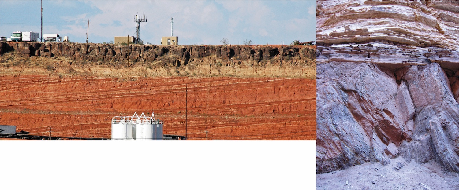
Superposition
- Trace out the rock layers on Figure 11.1 and number them, with 1 being the oldest.
- Are the rock layers the same thickness? Which rock layer is the thickest? Which is the thinnest?
- Are the rock layers constant thickness across the image? Can you explain why they are or are not?

Figure 11.1 – Sedimentary rock layers. Image credits: left: Pixabay, Public Domain; right: Wikimedia user Rhododendrites, CC BY-SA.
Original Horizontality
- On Figure 11.2, label the layers that are in their original position and those that are not.
- Are the rock types the lower and upper layers the same? Describe any differences.
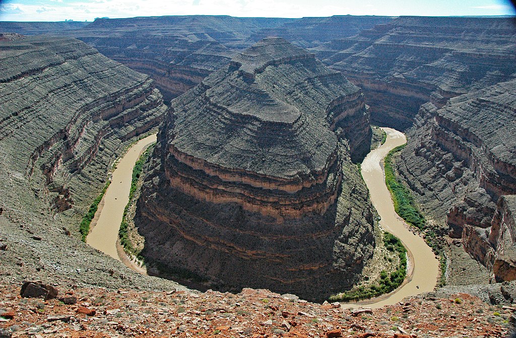
Lateral Continuity
- Connect the layers across the river on Figure 11.3.
- What types of rocks are shown?
- Why do some rock units have a vertical face while others have slopes?
Inclusions
- Which part of the rocks in Figure 11.4 are the inclusions? Circle them.
- Are the inclusions older or younger than their host rock?
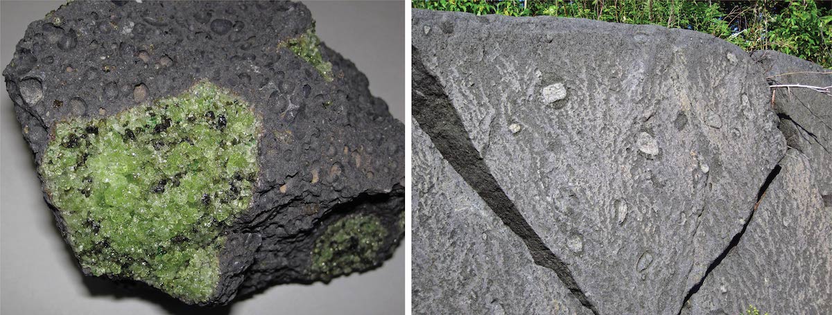
Figure 11.4 – Left: Peridotite mantle xenolith in a unique basalt from Arizona. Right: Metamorphic xenoliths in an ultramafic dike. Image credits: left, James St. John, CC BY; right, James St. John, CC BY.
Cross-Cutting Relationships
- In Figure 11.5, use cross-cutting relationships to determine which rocks are older.
- How many generations of igneous rocks are there in each photo?
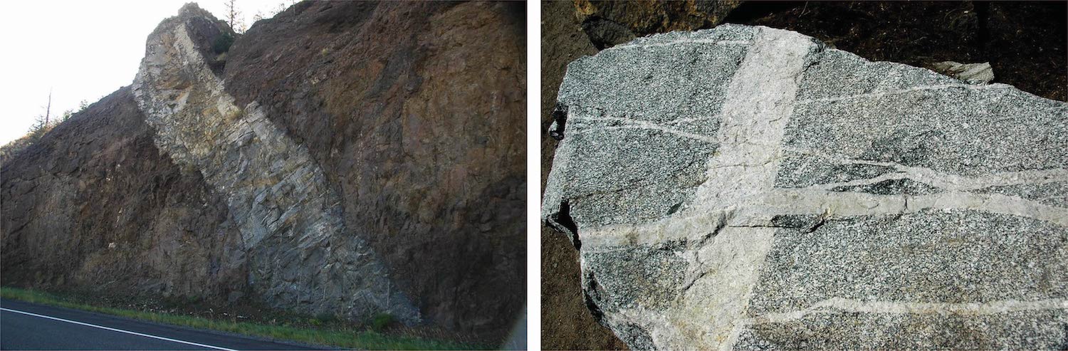
Figure 11.5 – Left: Andesite dike from Wyoming. Right: Felsic dikes and diorite from California. Image credits: left, James St. John, CC BY; right, James St. John, CC BY.
11.2 Unconformities
The geologic record is not like a video recorder that documents every single event in Earth’s history. There are times when nothing significant happens in the geologic time record, or the record is “deleted”. If there is erosion during this time, this leaves a time gap or unconformity; a contact between two rocks that represents a period of erosion. This means that even though the rocks touch each other, there is a difference in age. Sometimes the erosional surface will develop a soil layer and sometimes it is just rock. So, you can look for soil on the surface to determine if there has been a gap in time.
Simply speaking, an unconformity is a pattern that you look for in a group of rocks that tells you erosion has taken place. Rocks exposed on the Earth’s surface are affected by physical and chemical weathering processes that work to break them into smaller pieces or dissolve them in water. This material is then transported away by wind, water, or ice, a process known as erosion. Many people use weathering and erosion interchangeably, but they do mean different things: weathering is the breakdown of rocks, while erosion removes the broken down material.
There are three types of unconformities well focus on, and each forms in a slightly different way. They all involve sedimentary rocks, changes in sea level, and/or uplift from an orogeny. Each unconformity tells a unique story of the geologic history of the area they’ve been found.
- A disconformity is an erosional surface where the rocks below the unconformity are much older than the rocks above. This type of unconformity typically forms when horizontal layers of sedimentary rock are deposited in a shallow marine environment; then sea level lowers to expose these rocks and allows erosion to occur; then sea level rises again, and new horizontal layers of sedimentary rock are deposited. Erosion removed some of the original rock, creating a large age gap between the rocks above and below the erosional surface.
- A nonconformity forms when igneous or metamorphic bedrock is eroded, and then horizontal layers of sedimentary rock are deposited directly on top of it. The unconformity is where the bedrock meets the sedimentary rock. For example, when a mountain belt is eroded below sea level, and afterward sediments are deposited on top of the igneous or metamorphic rock.
- An angular unconformity is created when horizontal layers of sedimentary rock lie on top of tilted layers of sedimentary rock. For this to occur, sedimentary rocks deposited in the marine environment are lifted above sea level by a tectonic event ,which causes the sedimentary rocks to become tilted or folded. Since these rocks are exposed above sea level, erosion takes place. The rocks can either be eroded below sea level, or sea level can rise, which would allow new, horizontal layers of sedimentary rock to be deposited on top of the titled ones. This creates an angle between the younger, horizontal layers on top and the older, tilted layers below.
Exercise 11.2 – Looking at Unconformities
Unconformities can be confusing and difficult to identify if you are not an experienced geologist. Look at the following 3D models of unconformities. Investigate the labels and explore these outcrop models.
Now that you have seen some unconformities in outcrop, you can work to identify them on your own. The four models below are unlabeled outcrops with an unconformity. Take your time to study the outcrop, then make a quick sketch of each outcrop in Table 11.1, making sure to identify the unconformity. Do not worry about your sketches looking perfect. Sketches should take about a minute each and should only capture the essential features of the outcrop.
Model 1
Model 2
Model 3
Model 4
| Model 1 Sketch: | Model 2 Sketch: |
| Model 3 Sketch: | Model 4 Sketch: |
Now, you can use all of the principles you’ve learned to interpret the geologic history of a region. You’ll need to look for all events including metamorphism, igneous rocks, deformation (both folding and faulting), unconformities, and sedimentary units. If possible be specific about types of events such as normal faults, mafic dikes, nonconformities, etc. Also, don’t forget about the surface. Most geologic histories end at present day with formation of a landscape that may include erosion, volcanoes, rivers, and lakes. For example, in Figure 11.6, you can see a landscape in the map view that you would not imagine is hiding a complex geological history underneath:
- The sequence of geological events starts with a protolith, which is metamorphosed and folded into a high-grade metamorphic gneiss (rock A) at depth.
- Next, the gneiss is lifted towards the surface and displaced by a brittle fault (GF). Since the hanging wall is moving upward and the fault is at a shallow angle, this is a thrust.
- Both the gneiss and fault A are crosscut by an igneous granitic intrusion (rock B); its irregular outline suggests it was emplaced as magma into the gneiss. Since igneous rock B cuts both the gneiss and fault, igneous rock B is younger than these.
- Next, the gneiss A, fault GF, and igneous rock B were exposed at the Earth’s surface and eroded forming a nonconformity indicated with the wavy line (CU). This created an ancient landscape surface on which sedimentary rock E was deposited.
- Next, igneous basaltic dike D cut through all rocks except sedimentary rock I. Since, the top of dike D is level with the top of layer C, this establishes that erosion flattened the landscape prior to the deposition of layer I, creating a disconformity (JU) between rocks D and E.
- Fault HF cuts across all of the older rocks A, B, E and I, producing a fault scarp, which is the low ridge on the upper-left side of the diagram. This is a normal fault as the hanging wall moved downward.
- The final events affecting this area are erosion of the land surface, rounding off the edge of the fault scarp, and producing the modern landscape with a river cutting across the landscape.

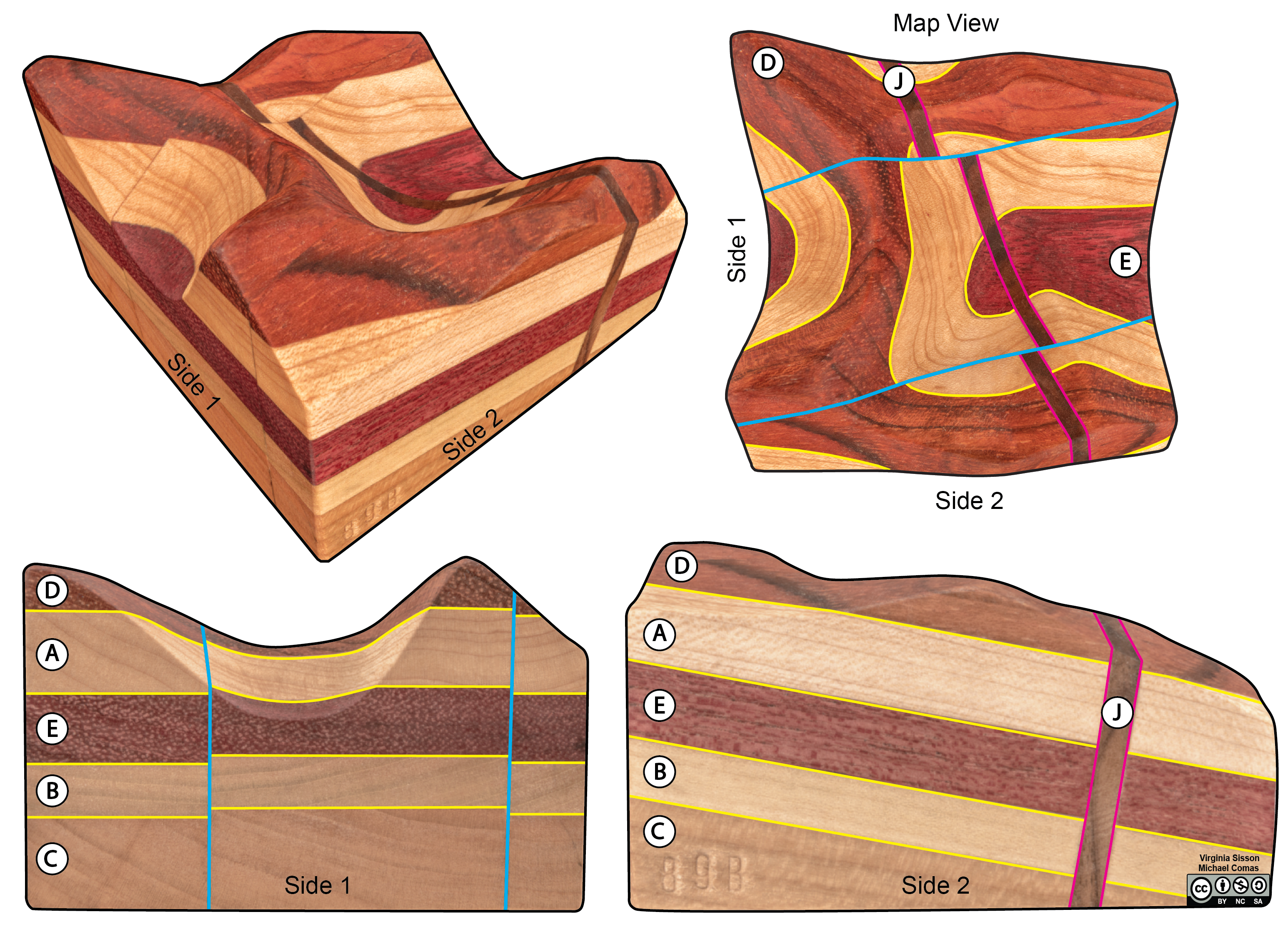
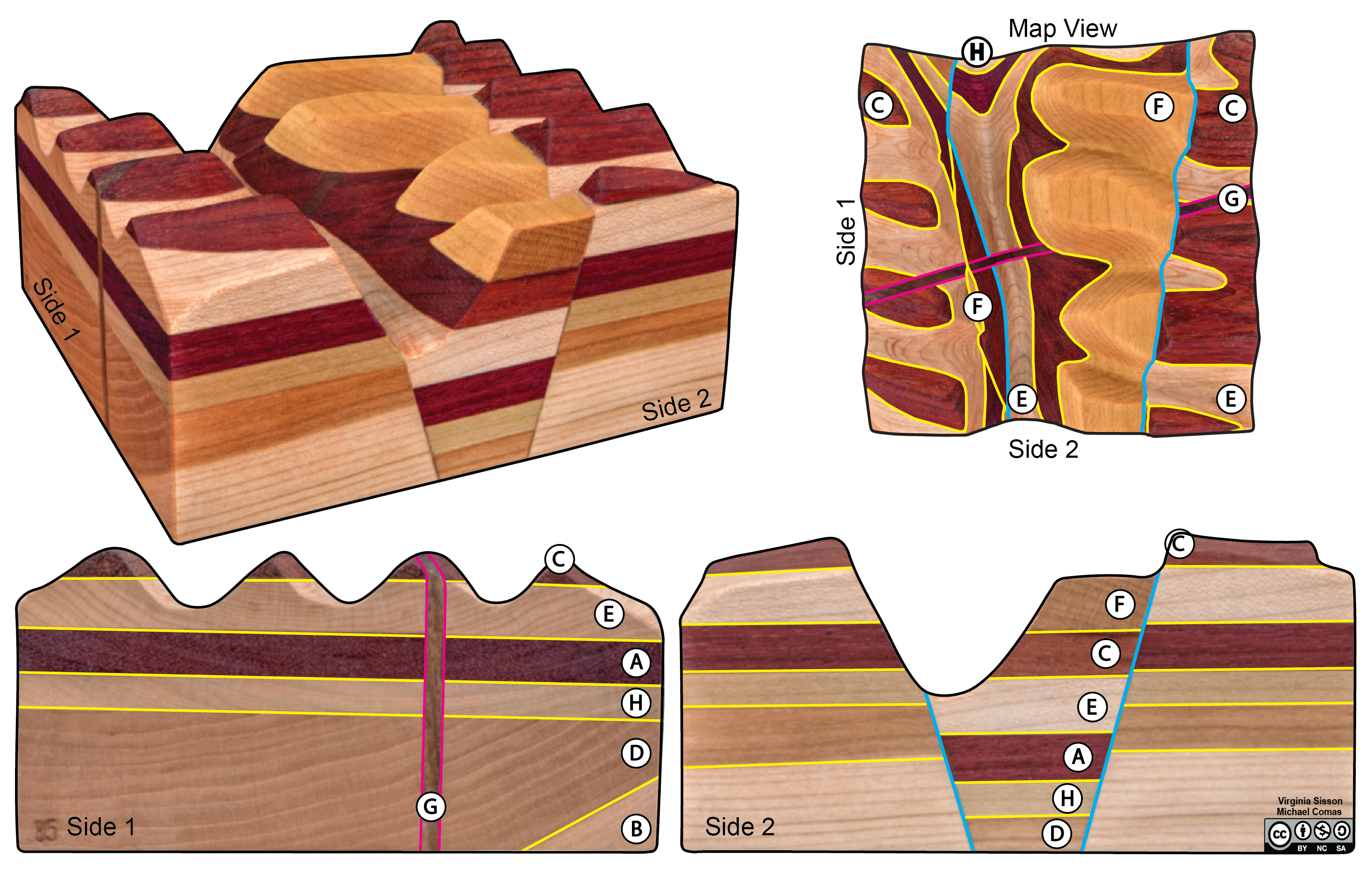
Exercise 11.3 – Sequencing of Geologic Events
Below are several diagrams that represent stratigraphic sections of rock each with a different geologic history. Now be a rock detective and figure out the sequence of events. Each letter represents the deposition of a different layer of sedimentary rock, igneous dike, or geologic event.
- Determine the order of events for the block model in Figure 11.7. Subscripts: F=folding, D=dike, U=unconformity. Hint: it is easier to start with the oldest event or rock unit and work your way forward through time.
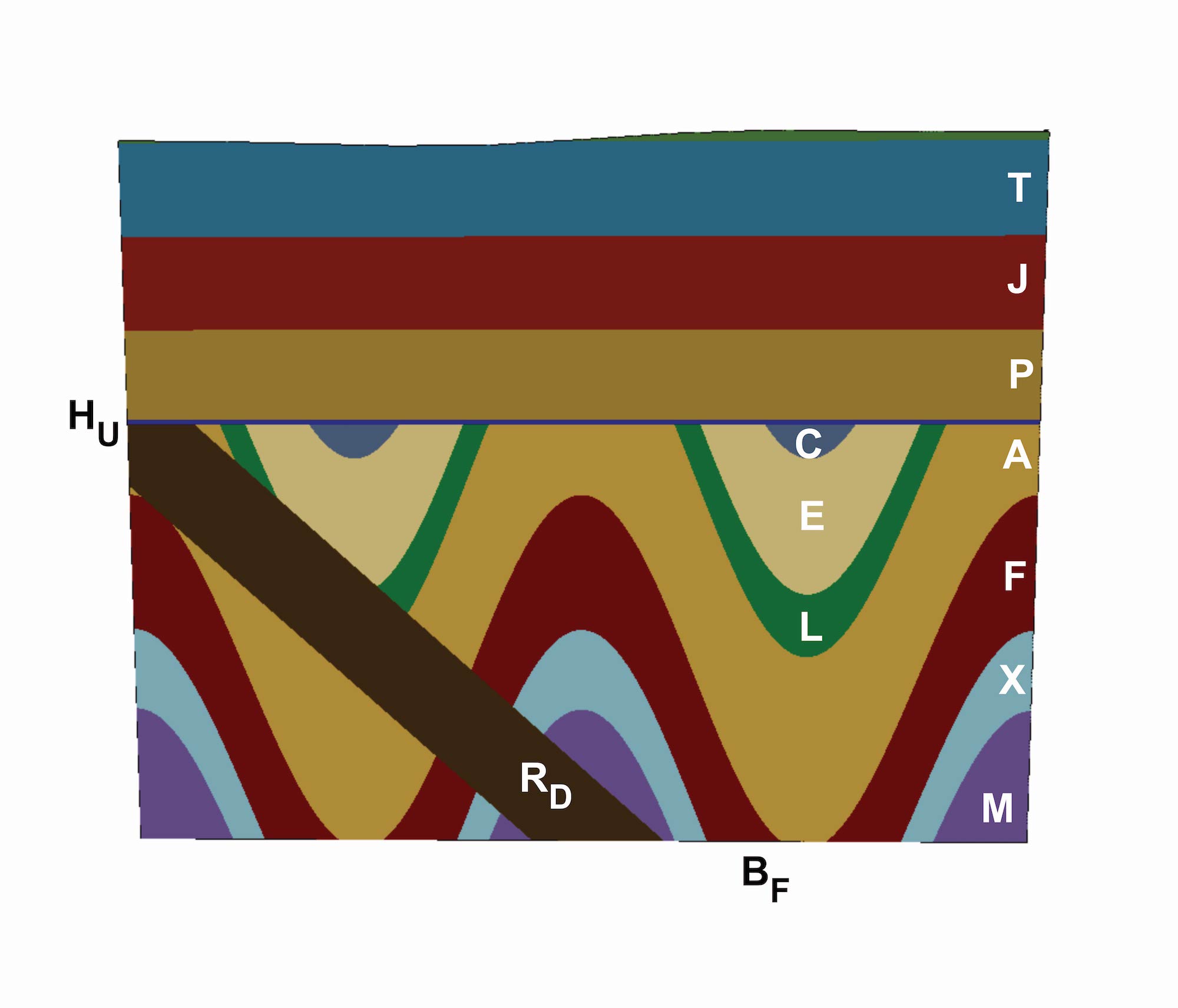
Figure 11.7 – Block model for relative dating created using Visible Geology. Image credit: Virginia Sisson CC BY. - The wooden block model in 11.8 shows several layers of sedimentary rock, a dike, and two faults. Determine the order of events for this block.
- Observe the two faults. Give their fault type and sense of motion
- Did you learn the Rule of Vs in either Chapter 11 Maps or Chapter 9? In the map view, compare the contacts of the different sedimentary layers shown in yellow to the contacts of the faults and dike. Which are straight versus curved? Why?

Figure 11.8 – Wooden block model of a fault (block 89b). Letters represent different layers of wood. Yellow lines are contacts between types of wood representing different sedimentary units. Blue lines indicate faults. Magenta lines indicate mafic dikes. One view is down a corner with map view and two sides. Also shown are a map view, side 1 and side 2. Since the wooden block has been carved to look like a land surface, the edges of the map view are not straight. Image credit: Virginia Sisson and Michael Comas using wooden block models created by Kurtis C. Burmeister with photogrammetry by Ryan Hollister CC BY-NC-SA. - The wooden block model in 11.9 represents a rift or graben. Use Figure 11.9, determine the order of events for this block.
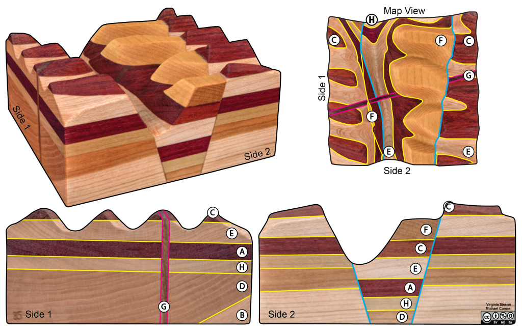
Figure 11.9 – Wooden block model of a graben (block 85). Letters represent different layers of wood. Yellow lines are contacts between types of wood representing different sedimentary units. Blue lines indicate faults. Magenta lines indicate mafic dikes. One view is down a corner with map view and two sides. Also shown are a map view, side 1 and side 2. Since the wooden block has been carved to look like a land surface, the edges of the map view are not straight. Image credit: Virginia Sisson and Michael Comas using wooden block models created by Kurtis C. Burmeister with photogrammetry by Ryan Hollister CC BY-NC-SA. - Critical Thinking: Erosion by rivers carves out valleys with the elevation getting lower downstream. Using your geologic history and the map view, which way was a river flowing: toward E or H? Explain.
11.4 Absolute Dating
Geologists can determine numerical ages for the formation of rocks, minerals, and some fossils using radioactive isotope systems. Does radioactivity sound scary? It can be, but what we’re talking about is happening on such a small scale that you don’t have to worry. The next few paragraphs are a bit technical, but we will try to break it down for you.
An isotope is an atom of an element with a different number of neutrons than protons in its nucleus. For example, a typical carbon atom on the periodic table of elements should have six protons and six neutrons in its nucleus, called carbon-12. Some atoms of carbon can have an extra neutron in the nucleus, called carbon-13, and some can have two extra neutrons in the nucleus, called carbon-14. If an atom has too many neutrons in its nucleus, it can become unstable because the nucleus has too much energy; this is called a radioactive isotope. Carbon-14 is a radioactive isotope.
Radioactive isotopes decay to more stable atoms by way of alpha, beta, and/or gamma decay. In short, radioactive atoms can gain or lose protons, neutrons, and electrons or release energy in other forms to become stable. For example, carbon-14 radioactively decays to nitrogen-14, a stable product. This ThoughtCo article gives a very simple explanation of why atoms become radioactive if you want more information.
| Parent Isotope | Stable Daughter Product | Half-life |
| Uranium-238 | Lead-206 | 4.5 billion years |
| Uranium-235 | Lead-207 | 704 million years |
| Thorium-232 | Lead-208 | 14.0 billion years |
| Rubidium-87 | Strontium-86 | 48.8 billion years |
| Potassium-40 | Argon-40 | 1.25 billion years |
| Samarium-147 | Neodymium-143 | 106 billion years |
| Carbon-14 | Nitrogen-14 | 5,730 years |
Radioactive isotopes don’t all immediately decay to a stable form because it’s a spontaneous process, so it’s impossible to predict when and which atom will decay. It’s like corn kernels popping in a popcorn maker, you don’t know when a kernel will pop, but you know it will happen. Scientists have measured the average rate for radioactive decay and call this half-life. Half-life is the time it takes for half of the unstable atoms (parents) to decay to stable forms (daughters) (Table 11.2). For example, the half-life for carbon-14 is 5,730 years, but the half-life for potassium-40 is 1.25 billion years. In a sample with 1 million atoms of carbon-14, 500,000 of these atoms are expected to decay over 5,730 years.
Geologists analyze a material’s chemistry and figure out the ratio between parent and daughter atoms. This ratio tells geologists how many half-lives, or what fraction of a half-life, has passed. If you know this ratio and the rate of decay for that isotope system, you can calculate how old geologic material is.
The symbols ka (thousands), Ma (millions), and Ga (billions) refer to points in time like a date. For example, the dinosaur extinction occurred at 66 Ma. Geologists also use other abbreviations for lengths of time, including ky, kya, kyr, and k.y. for thousands of years; my, mya, myr, and m.y. for millions of years; and by, bya, byr, and b.y. for billions of years. All four varieties of abbreviations mean the same thing in this case. Here, you would say the dinosaurs have been extinct for 66 myr. If this sounds confusing, you’re not alone because even some geologists use all of the abbreviations interchangeably.
Exercise 11.4 – Absolute Dating
For the exercise, your instructor will provide you with a container of marbles. This is an analog for a mineral that we want to determine the age that it formed. Select two colors to work with. One color will be your parent radioactive isotope and the other will be the stable daughter product.
- Parent (P) Color: ___________________
- Daughter (D) Color: ____________________
- Number of P “atoms”: __________
- Number of D “atoms”: __________
To calculate an age, use the age equation: t = [ln((P+D)/P)]/λ
- t = time
- P = number of parent atoms
- D = number of daughter atoms
- λ = is the decay constant (different for every isotope system)
- How old is your mineral if λ is 1.21×10⁻⁴? ____________________
- Critical Thinking: Recall the exercise on accuracy and precision from the first chapter. Do you think your answer is precise? How many marbles would you need to count to get a better precision?
- Critical Thinking: Compare your result with those of your class. What is the range of ages? If these geologic samples, how would you interpret this data?
11.5 Using Geologic Dating
Absolute dating tells you different things depending on which rock type you are studying. For minerals in igneous rocks, the radiometric age tells you when the mineral crystallized from magma. In metamorphic rocks, the radiometric age of some minerals can give you the age metamorphism took place, but some isotope systems are not affected by metamorphism and can still tell you the age the minerals originally crystallized in the protolith. So, you can determine when the protolith formed and when it became metamorphosed. Other minerals in both igneous and metamorphic rocks, do not retain their daughter isotopes until the mineral has cooled below a certain temperature. This gives you the age the rock cooled below that temperature.
For minerals in sedimentary rocks, the radiometric age only tells you when that mineral crystallized or metamorphosed in its original rock; it doesn’t tell you when the sedimentary rock formed. The only way to determine the age of sedimentary rocks is to combine the principles of relative dating with radiometric dating of igneous or metamorphic events that crosscut the sedimentary rocks, such as a dike. Ages of sedimentary rocks can also be determined from fossils.
Relative and absolute dating methods can be useful for developing the stratigraphic history of an outcrop, but when used together, they are even more powerful. For example, when scientists first discovered the famous Australopithecus afarensis hominin fossil skeleton nicknamed “Lucy” in Ethiopia, they initially estimated her age using the principles of stratigraphy and the occurrence of pig fossils between 3.5 and 2.9 million years ago. Then in 1992, absolute dating techniques were used on volcanic ash beds that were deposited 1 m below Lucy’s skeleton; these resulted in a more precise age of around 3.18 million years old. To further refine this age, we can use local sedimentation rates of 14 to 30 cm per 1000 years. This means her age is closer to 3.15 to 3.12 Ma when she was fossilized. So, combining relative, fossil, and absolute age techniques can be beneficial to better constrain events on Earth.
Exercise 11.5 – Combining Dating Techniques
Figure 11.10 is a hypothetical outcrop view of several sedimentary units that have been deposited on top of a metamorphic bedrock. There are also three igneous events. The age of metamorphic rocks and igneous events can often be found by using radiometric dating methods, but the age of the sedimentary layers can only be determined through cross-cutting relationships with the igneous and metamorphic rocks.
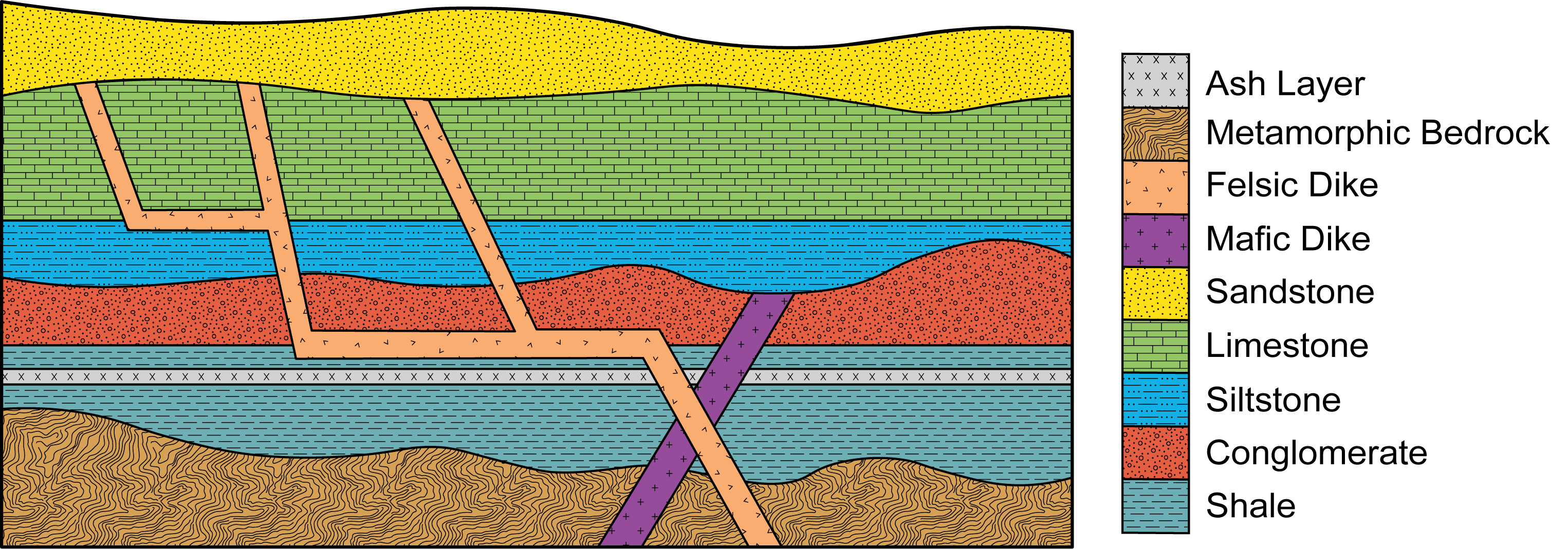
- Good news! You’ve already collected samples from the igneous and metamorphic events to determine their ages. Complete the calculations for each. To calculate an age, use the age equation: t = [ln(P+D/P)]/λ.
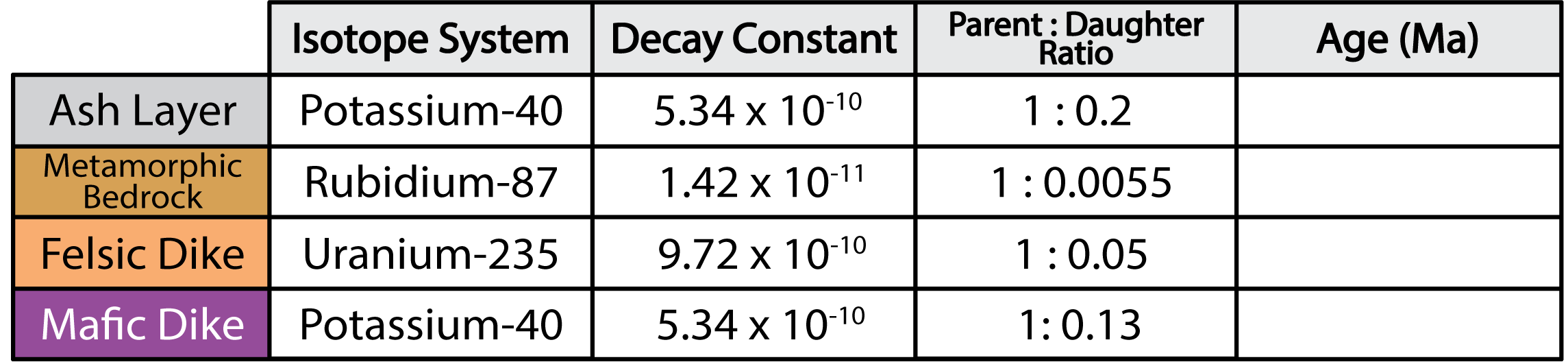
Figure 11.11 – Calculations for the igneous and metamorphic rocks. - Now that you know the age of the igneous and metamorphic events, determine the minimum and maximum ages for the sedimentary layers and what time periods they are from.
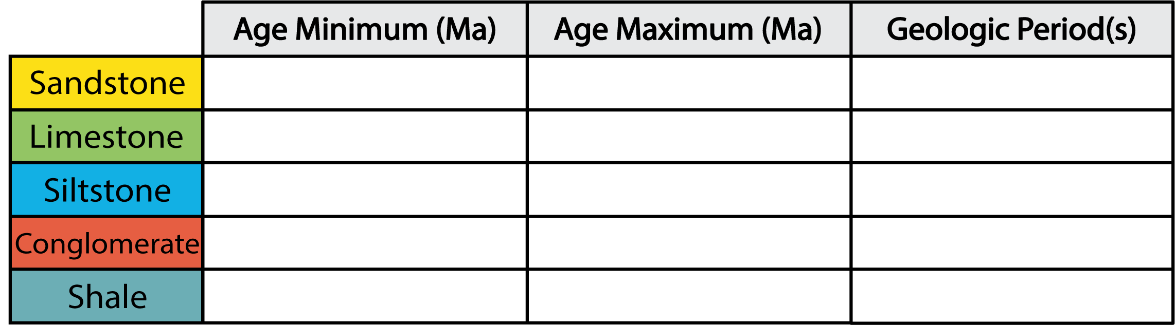
Figure 11.12 – Determining the age ranges for the sedimentary rocks. - What are the approximate ages of the four unconformities (indicated by the wavy lines)?
- Now that you have ages for all the events place them in order from oldest to youngest. Determine the order of events for this outcrop.
- Do you think the unconformity above the metamorphic bedrock formed relatively soon after the rock’s formation or long after?
While topographic maps are useful for looking at topography, often times geologists are interested in the geology of a region. A geologic map is a type of map that provides information on the geologic features and formations of a particular area. It can be used to understand the distribution, composition, and relationships of rocks, minerals, and other geologic features. Additionally, you can use a geologic map to deduce the area’s geologic history.
Geologic maps use various colors, patterns, and symbols to represent different rock types or rock units, geological formations, faults, folds, and other geologic structures. Key elements commonly found on geologic maps include rock units, stratigraphic formations, folds and faults, and topography.
Exercise 11.6 – Age relations on a geologic map
Figure 11.13 highlights the different parts that are common on geologic maps. These include the map, cross-sections, explanation of units, scale, location, etc. This map also has locations for economic mineral deposits including silver-lead mines. In this region, over 15 million ounces of silver were produced from 1875 to 1957. Your instructor may provide you with a printed version of the USGS map. Answer the following questions.
- Where is this map located in the U.S.?
- What is the oldest unit represented on this map? Use the legend to help.
- What type of rock is the oldest unit? Be specific and not just igneous, metamorphic or sedimentary.
- What is the youngest unit represented on this map?
- Describe the geology of the youngest geologic formation.
- What is the dominant rock type in this region?
- Name the geologic structure at the top-center of the map in the Colorado, Kootenai, and Morrison and Swift formations.
- What is the general trend of the anticlines and synclines in this area? Using the orientation of these structures, what was the orientation of convergent forces?
- Locate cross-section B-B’. What are some geologic features in this cross-section?
- Locate the Sagebrush Park stock. This is a granodiorite and quart diorite intrusive igneous rock. Did the intrusive body intrude into the country rock before or after folding?
k. Critical thinking: On the western side of the map, there is another suite of igneous rocks, the Elkhorn volcanics. Are they younger or older than the Sagebrush Park stock? What additional information could you use to determine their age relations?

Even though radiometric dating of sediments isn’t useful for determining the age of sedimentary rocks, the ages are useful for determining which rocks the sediments were eroded from. This is called provenance. One method for understanding depositional patterns in evolving sedimentary basins is to conduct detrital zircon (DZ) geochronology on different layers. This absolute dating method uses the ages of zircon grains within sandstones to tell how sediment sources changed through time. DZ ages are found by using a mass spectrometer to compare the ratios of radioactive lead and uranium within zircon grains.
As you may have notice in Table 11.2, most radioactive elements have only one parent and daughter. This is not true for uranium (U) as it has two parallel decay schemes with 238U and 235U parent isotopes and a multi-step decay to daughter elements (206Pb and 207Pb). So, instead of using the decay equation, geoscientists use a plot of 206Pb/238U against 207Pb/235U for concordant samples of various ages should define a single curve, named ‘concordia’ by G. W. Wetherill in 1956. For more on U-Pb geochronology, click on this link.
How to measure all these different isotopes for determining mineral and rock ages? Use a mass spectrometer which can measure the mass of a molecule by measuring the mass-to-charge ratio (m/z) of its ion. This technique was first used in 1918 and over the years, two Nobel Prizes have been awarded for advances in mass spectrometery. In the 1950’s, geologists first started using this technique for U-Pb analysis. What is the future of this technique? Well, NASA is developing mass spectrometers to go into space (Figure 11.15). So, perhaps we’ll be able to remotely do geochronology and determine more about the history of our solar system.

Exercise 11.7 – Sediment Provenance
In east-central Texas, the Paleocene Wilcox Group consists of sandstones that house important resources including aquifers, lignite coal and petroleum. To better understand this sediment, you have been tasked with determining its geologic history of an east-central Texas study area (Figure 11.15) using detrital zircon (DZ) geochronology. The U-Pb method of dating is the one usually applied to zircon. This method relies on two separate decay chains, 238U to 206Pb, with a half-life of 4.47 billion years, and 235U to 207Pb, with a half-life of 710 million years.
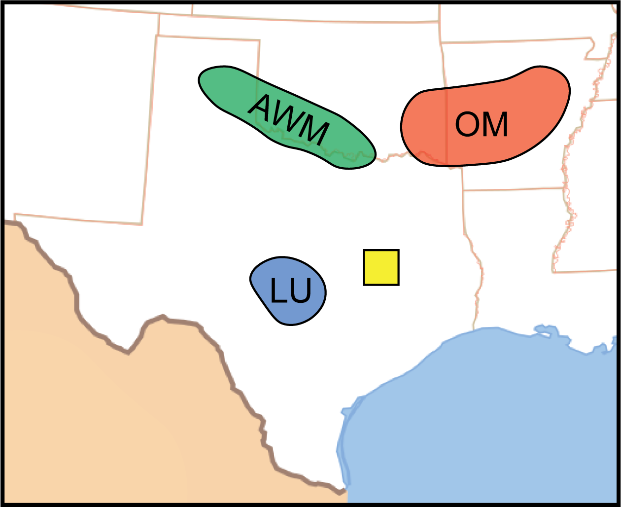
- The first step is to determine the age of the source areas. You’ve already collected samples from each source and determined their U/Pb ratios (Table 1.3). Use Figure 11.16 to determine the ages of your source areas.
Table 11.3 – U-Pb isotope data for source rocks Region 207Pb/235U 206Pb/238U Age (Ma) Amarillo-Wichita Mountains 7.5 0.3 Llano Uplift 4.5 0.25 Ouachita Mountains 0.5 0.05 
Figure 11.16 – Wetherill concordia diagram for U-Pb. Image credit: Michael Comas, CC BY-NC-SA. - A sandstone from the study area contains many zircon grains with U/Pb ages of ~1100 Ma. Where were these sediments mainly sourced from?
- The unit above the sandstone shows U/Pb ages of ~300 Ma. Why do you think these two adjoining units have zircon grains of different ages?
- Propose and explanation for what caused the change.
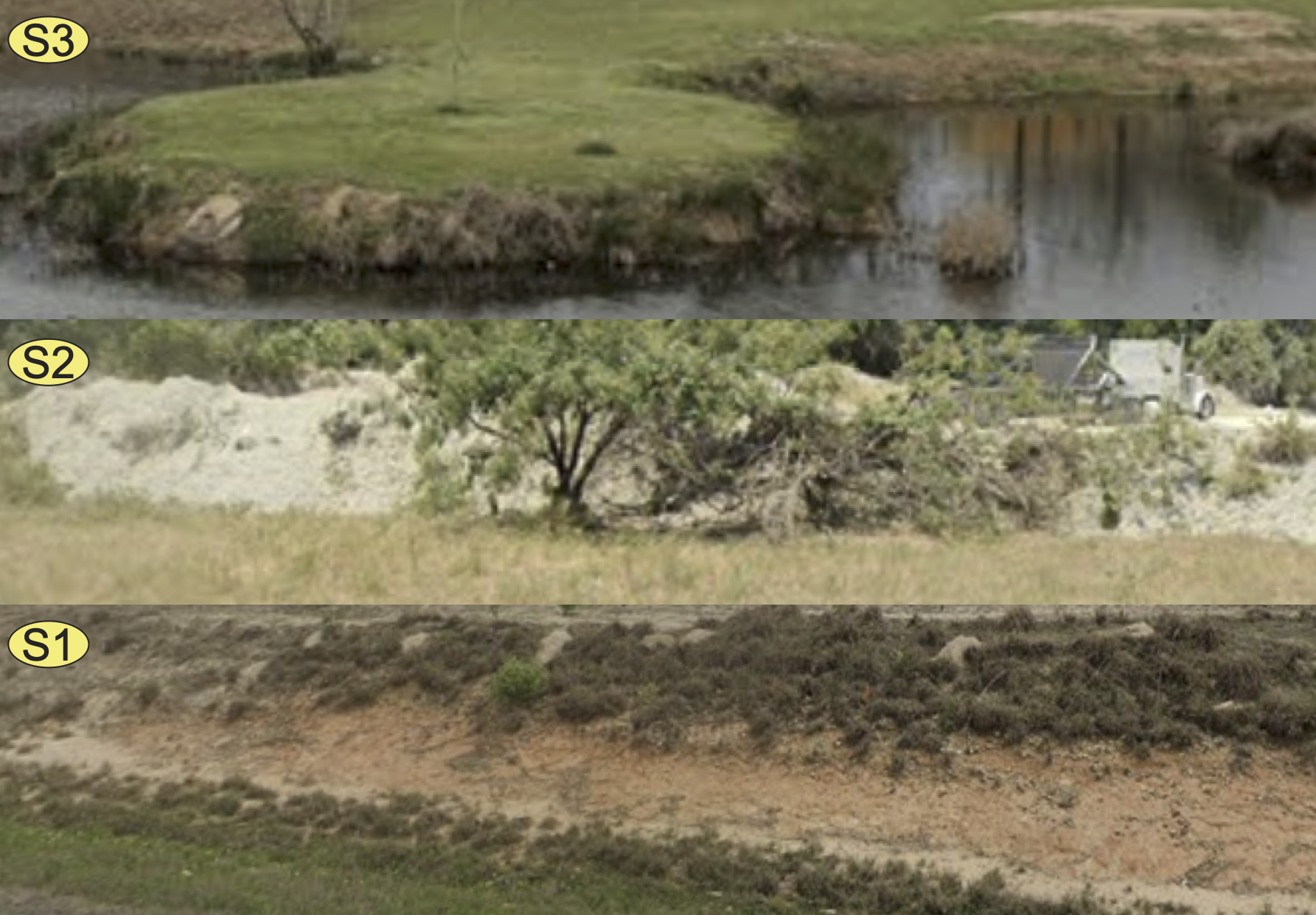
- Figure 11.17 is a series of photos from the study area that shows outcrops of the Wilcox Group with fine-grained sandstone. Three sandstone layers have been selected (S1, S2, S3) to determine the provenance of the sediment. Age data from hundreds of zircon grains has been collected and presented in Figure 11.18. Reconstruct the depositional history of these sediments that including where they are sourced from, and an explanation for why sources may have changed through time. The potential source areas remain the same as those you looked at earlier in Table 11.3.
- Critical thinking: These sample sites are all in drainage basins of paleorivers. These paleorivers collected sediment from the various source areas. Draw the paleorivers on Figure 11.15. How do you think the paleorivers evolved through time?

Additional Information
Exercise Contributions
Michael Comas, Virgina Sisson, and Daniel Hauptvogel
References
Klepper, MR, Weeks, RA, and Ruppel, ET, 1957, Geology of the southern Elkhorn Mountains, Jefferson and Broadwater Counties, Montana, U.S. Geological Survey Professional Paper 292 doi:10.3133/pp292
Wahl, P.J., Yancey, T.E., Pope, M.C., Miller, B.V., and Ayers, W.S., 2016, U-Pb detrital zircon geochronology of the Upper Paleocene to Lower Eocene Wilcox group, east-central Texas, Geosphere, v. 12, p. 1517-1531. DOI:10.1130/GES01313.1
a method to determine the order of past events by comparing the ages of different geological events
a method of determining the numerical age of rocks. Absolute dating uses isotopic measurements to calculate the time elapsed between a rock-forming event and the present.
a type of geologic contact-a boundary between rocks usually caused by a period of erosion. It can also by a significant pause in sediment deposition
an elongated block of the Earth's crust lying between two normal faults that has been displaced downward

_2_(20634177933).jpg#file)