
Chapter 13: Landscapes
Learning Objectives
The goals of this chapter are to:
- Understand forces that change the landscape in different environments
- Interpret rates of change of landscapes
- Evaluate the impact of landscape changes on humans
13.1 What is Geomorphology?
Geomorphology (from Ancient Greek: geo “earth”; morphe, “form”; and logos, “study”) is the scientific study of the origin and evolution of topographic and bathymetric features generated by physical, chemical, or biological processes operating at or near Earth’s surface. Geomorphologists seek to understand why landscapes look the way they do, to understand landform and terrain history and dynamics, and to predict changes through field observations, physical experiments, and numerical modeling.
Many forcing agents control the shapes of landscapes, with streams being the dominant force in most continental regions. Other forces include gravity, wind, glaciers, oceans, wildfires, people, and even water beneath the surface. Also important is climate – more about that in Chapter 15.
Exercise 13.1 – Observing Landscapes
Look at various landscapes and notice their geomorphologic features
- Figure 13.1 is a photo from Death Valley in California. Describe the landscape features that stand out to you.
- How do you think these features may have formed?
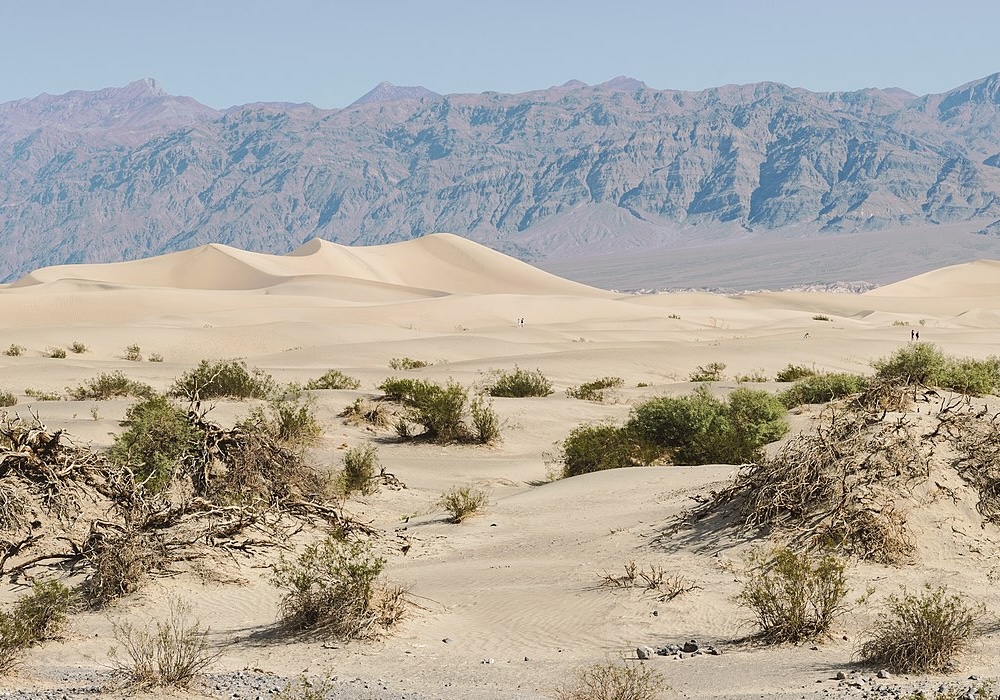
Figure 13.1 – Death Valley, California. Image credit: Tuxyso, CC BY-SA. - Figure 13.2 shows a valley in Yosemite National Park, also in California. Describe the landscape features that stand out to you.
- Take a look at the valley in the center. How do you think it formed?
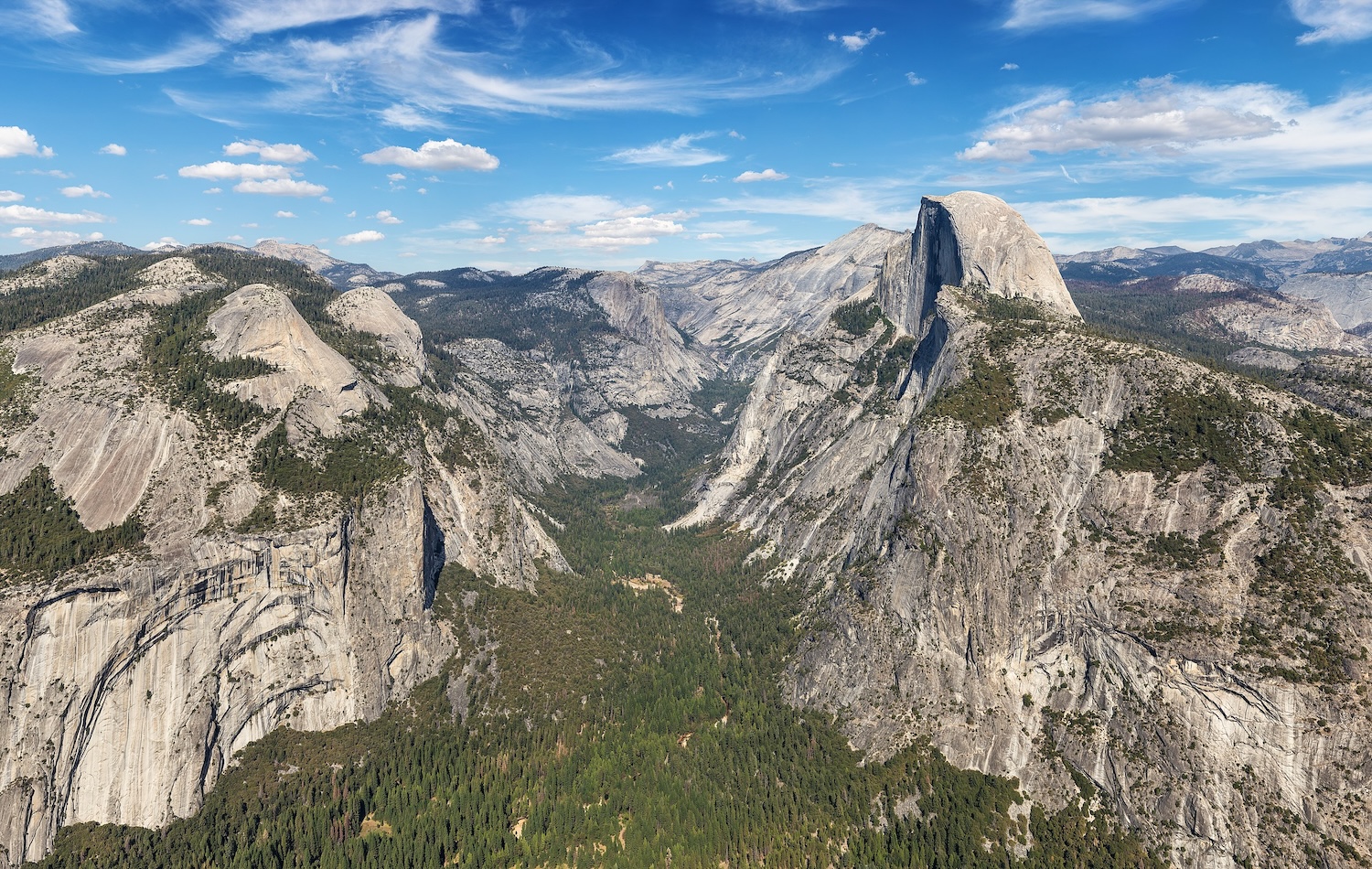
Figure 13.2 – Yosemite Valley in Yosemite National Park, California. Half Dome is on the right side of the valley. Image credit: Thomas Wolf, CC BY-SA. - Figure 13.3 shows the Li River in China. Describe the landscape features that stand out to you.
- How do you think those rocky towers formed?
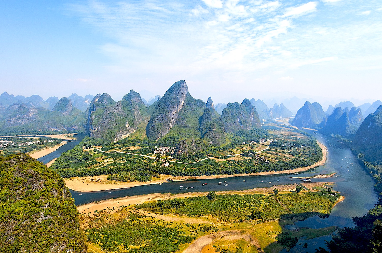
Figure 13.3 – Figure 13.2 – The Li River near Guilin, China. Image credit: Chensiyuan, CC BY-SA. - The landscape feature in Figure 13.4 is less apparent because it’s showing something on a large, regional scale. Based on the image and caption, describe what has happened.
- What could have caused this?
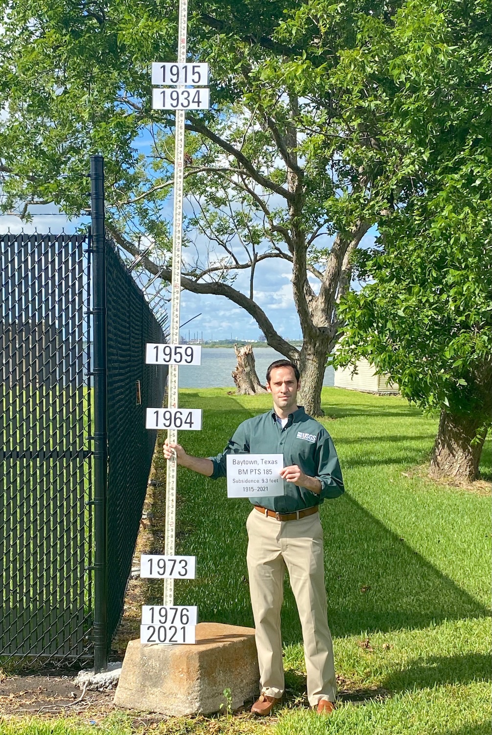
Figure 13.4 – The photo compares the elevation of the land surface from 1915 to 2021. The sign shows a difference of 9.5 feet. Image credit: USGS, Public Domain.
13.2 Desert Landscapes
The first landscape to explore is deserts, which are mainly affected by wind, and large sand dunes are a common feature. Desert sand dunes commonly form when there is an abundant sediment supply, and wind is strong enough to transport the sand. Dunes form where a dry climate prevents vegetation from interfering with their development. Sand dunes, however, are not restricted to deserts and can be found along seashores, along streams in semiarid climates, in areas of glacial outwash, and where sandstone bedrock disintegrates to produce an ample supply of loose sand.
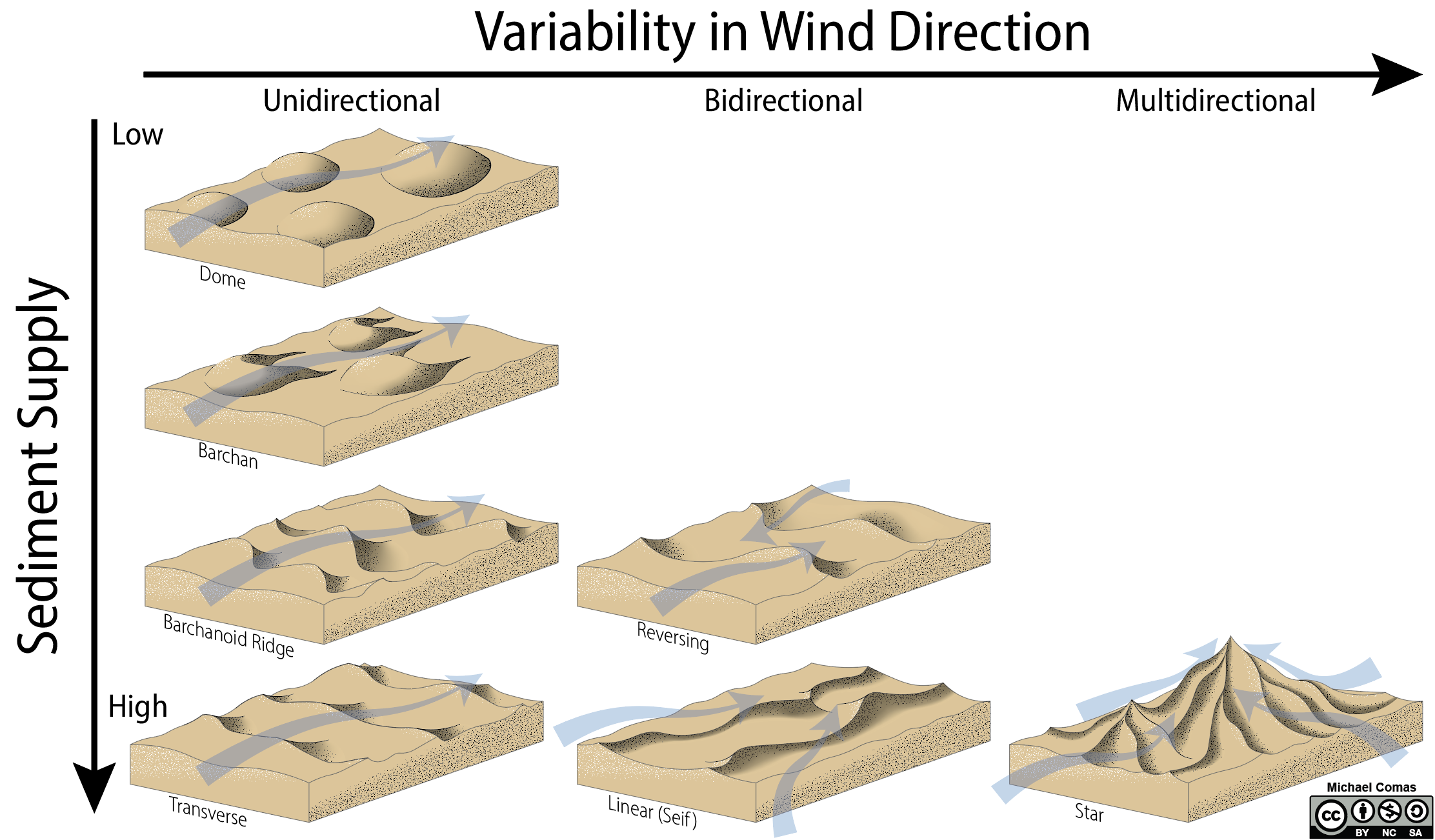
Two main factors dictate dune shapes: the amount of loose sediment and whether there is one or more prevailing wind directions. The strength, direction, and persistence of winds help determine how dunes develop. In some areas, winds will blow in one direction during the summer and another in winter. In other areas, there may be multiple wind directions. This variability in wind changes the shape of the dunes as well as their names (Figure 13.5). Sand is pushed or bounces (saltation) up the shallow side and then slides down the steep side (slip face). This characteristic shape is easy to see from a side view but harder to see in map view.
Vegetation acts as a barrier to wind, so sand may build up behind the vegetation. Vegetation also makes the sand surface rougher, which can affect sand movement. Also, deep roots can stabilize sand and prevent it from moving. These effects significantly impact sand dunes along the coast and at the edge of a desert where there is enough moisture for plants to grow.
Exercise 13.1 – Observing Sand Dunes
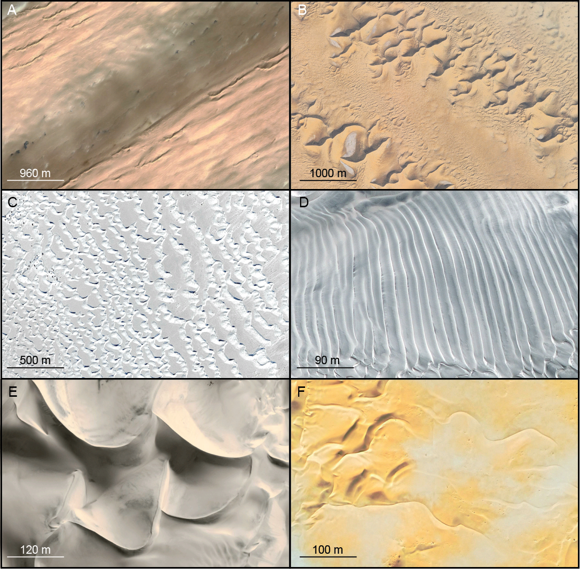
Figure 13.6 shows different types of sand dunes. Answer the following questions about them, and be sure to look at the scales on each image to get a sense of their size.
- Observe the similarities and differences between the dunes in each photo. Trace the crest of as many dunes as possible.
- For each image, describe the geometry of the dunes.
- Tenere Desert, Niger:
- Gran Desierto, Mexico:
- White Sands National Park, NM:
- Caravelli, Peru:
- Huachachina, Peru:
- Wadi Al Hajaa, Libya:
- Tenere Desert, Niger:
- On each image, draw arrows to indicate the wind direction(s). Some may have more than one prevailing wind direction.
- List the dunes in order of increasing sediment supply. Explain.
- What do you think gives the sands of White Sand Dunes National Park their color?
- Do you notice vegetation in any of these arid settings?
- How do you think vegetation affects dune formation?
- Critical Thinking: Why can dunes vary in shape at different scales?
Exercise 13.2 – Measuring Dune Migration
This movement of sand is emerging as a significant problem as desertification, or the process by which land becomes desert, is threatening about one fifth of the world’s lands. In fact, the United Nations has declared this to be our planets greatest environmental hazard and predicts over 50 million people will be displaced by this process in the next ten years.
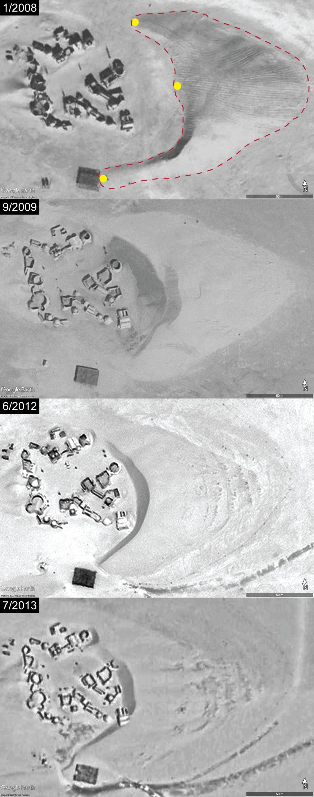
One of the filming locations for the Star Wars movie series was in the Saharan desert of Tunisia, where sand dunes migrate across the landscape. Since the set was built in 1976, it has been become a tourist attraction. Figure 13.7 shows four Google Earth images of the set from different times over a 5.5-year period. A single barchan dune is outlined with a red dashed line. A barchan dune is crescent-shaped and has a shallow side and a steep side. Wind transports sand up the shallow side of the dune, and sand tumbles down the steep side. Based on the images, you can see that the barchan dune is approaching the film set, which is a problem for this popular tourist attraction. Let’s figure out the rate at which this dune is moving.
- Three points of the dune have been marked with a yellow dot: the northern point, central, and southern point. Measure the distance that these points move between each time and fill this in on Table 13.1. It may help to outline the dune for each image.
Table 13.1 – Dune movement distance Time Period Northern Point (m) Central (m) Southern Point (m) 1/2008-9/2009 9/2009-6/2012 6/2012-7/2013 Total Movement - What is the dune movement rate for each part of the dune? The rate is distance/time. Fill this in on Table 13.2.
Table 13.2 – Rate of dune movement Time Period Northern Point (m/yr) Central (m/yr) Southern Point (m/yr) 1/2008-9/2009 9/2009-6/2012 6/2012-7/2013 - Why do you think there are different movement rates for the dune?
- What is the overall movement rate for each part of the dune over the 5.5-year period?
- Northern Point: ____________________
- Central: ____________________
- Southern Point: ____________________
- How long before each part of the dune makes it to the westernmost buildings of the film set?
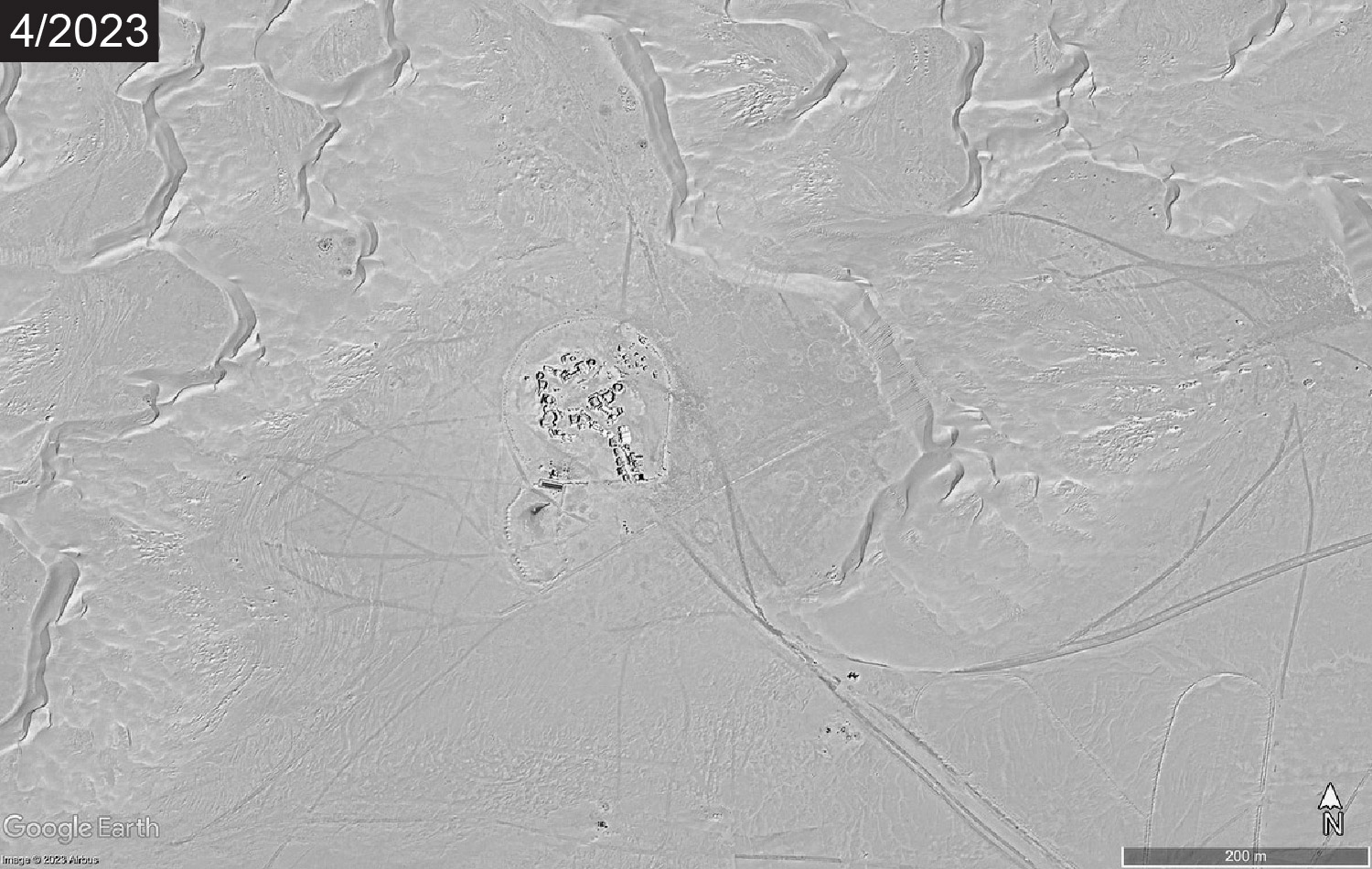
- Critical Thinking: Figure 13.8 is the latest image from the film set from 2023. What happened to the dune?
13.3 Glacial Landscapes
Next let’s explore glacial landscapes are where snow turns into dense glacial ice. A glacier is a body of ice that moves under its own weight. Currently, glacial ice covers about 10% of Earth’s land surface, mainly in Antarctica and Greenland. At various times throughout geologic history, glacial ice has been much more extensive, covering up to 90% of the Earth’s land surface. They are the largest repository of freshwater on Earth (~69% of all freshwater) and are highly sensitive to climate change. For mountainous regions, glaciers are an important source of drinking water.
There are two types of glaciers: alpine (found at high altitudes) and continental (found at high latitudes). The largest glaciers can cover entire continents and be several kilometers thick. Ice masses of this size leave behind very distinct features. As they advance, they carve through the surrounding landscape and transport sediment. As they retreat, large volumes of meltwater carry and deposit sediment. These carved or deposited features can tell scientists that a glacier used to cover an area and inform them about how the glacier behaved.
Many glacial features are very large, larger than what can be observed in a single outcrop. One way that geologists can interpret large-scale landscape features is through LiDAR imaging (Light Detection and Ranging). LiDAR is an imaging technique that can make a detailed elevation map of an area without tree cover.
Exercise 13.3 – Observing Glacial Landscapes
To observe some glacial features in LIDAR for yourself, first visit the Washington LIDAR Portal. Once you have entered the site, select “Hide All” towards the top of the page. Then scroll down the grey list of maps until you see “Island 2014” and select the box next to DTM Hillshade. After a second, you should see a greyscale digital hillshade model covering Whidbey Island in northern Puget Sound.
- Look at the southern half of Whidbey Island. Describe the pattern(s) you see in the landscape. It may help to zoom in to either 2 km or 1 km on the scale bar.
- How do you think these patterns could have formed?
- What can you infer about the ice flow direction in this area?
- Look to the far west side of the island, just west of Penn Cove. Describe the pattern(s) you see in the landscape. Zoom in to 100 m on the scale bar for the best view.
- What are these features?
- Look at the northern part of the island, northeast of Crescent Harbor. Describe the pattern(s) you see in the landscape. Zoom to 500 m on the scale bar for the best view.
- Where else on the island did you see these features? What are the differences in their orientation?
- How would you explain the difference in orientation?
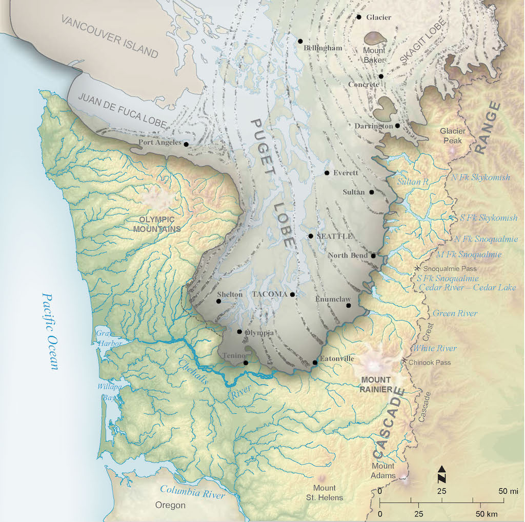
- Figure 13.9 shows the extent of the Puget Lobe of the Cordilleran ice sheet 16,000 years ago. Why do you think Mount Baker was not covered by the glacier?
- What about the area just south of Mount Baker?
Isostasy and Glacial Rebound
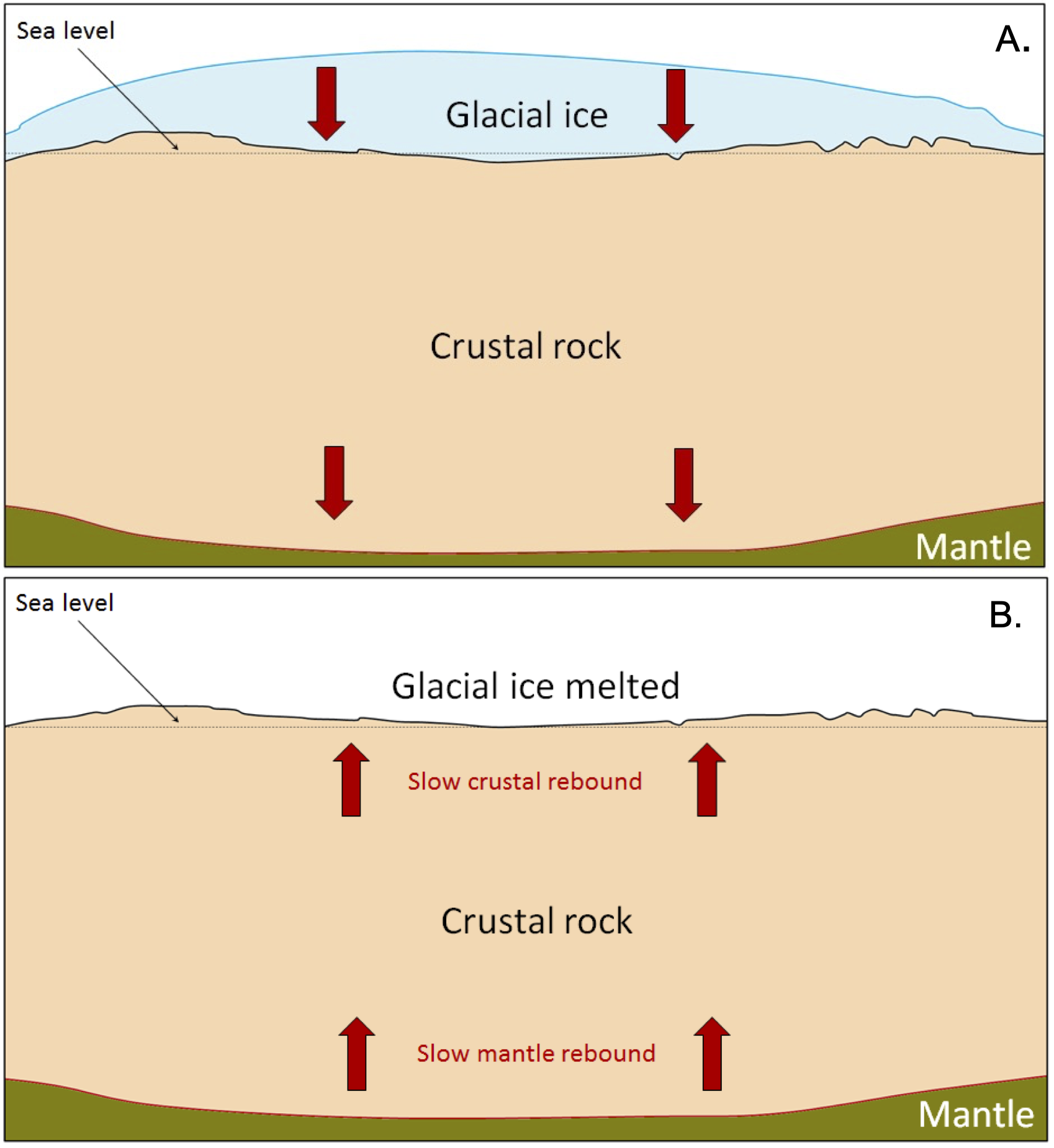
Another factor in understanding landscapes is the height of a region. In lecture, you may have been introduced to the concept of isostasy, or the principle that the Earth’s crust is floating on the mantle, like a raft floating in the water. Isostasy also applies to high topography in mountainous regions. As erosion reduces the height, the weight of the crust decreases, and it rebounds. This same principle applies to glaciers, as thick glacial ice adds weight to the crust and causes the crust to subside. For example, the Greenland Ice Sheet is over 2,500 m thick, and the crust beneath the thickest part has been depressed to the point where it is below sea level over a wide area (Figure 13.10). The same is true in parts of Antarctica. When the ice sheet melts, the crust and mantle will rebound.
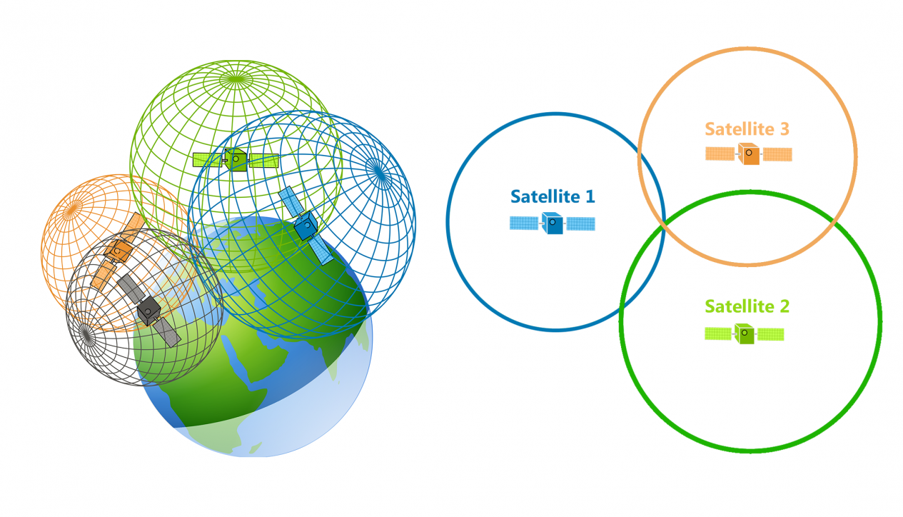
To measure Earth’s movements, geoscientists use high precision global positioning satellites (GPS) instruments. You probably have used the GPS in your mobile phone to get you where you want to go. Most of the time, you don’t have to pay attention to the vertical data from the GPS unless you are on a hike and need to know if you are the correct elevation. So, how does the GPS get elevation data? A GPS uses trilateration to find location information. This uses overlapping spheres instead of overlapping circles to determine location (Figure 13.11). In general, the more satellite data, the more precise and accurate your location will be calculated.
Exercise 13.4 – Glacial Rebound
Greenland is the world’s largest island located between the Arctic and Atlantic oceans and is covered by a large ice sheet. This vast body of ice covers 1,710,000 square km (660,000 sq mi), roughly 80% of the surface of Greenland. Recent estimates are that 1,034 billion metric tons of ice was lost from 1985 to 2022. This ice has a minimal effect on sea level causing and increase of 0.5 mm. More importantly, it has introduced lots of cold and fresh water to the northern oceans (Greene et al., 2024). So, how is the landscape of Greenland reacting to this change. According to isostatic rebound theory, it should be going up. Now let’s check this hypothesis.
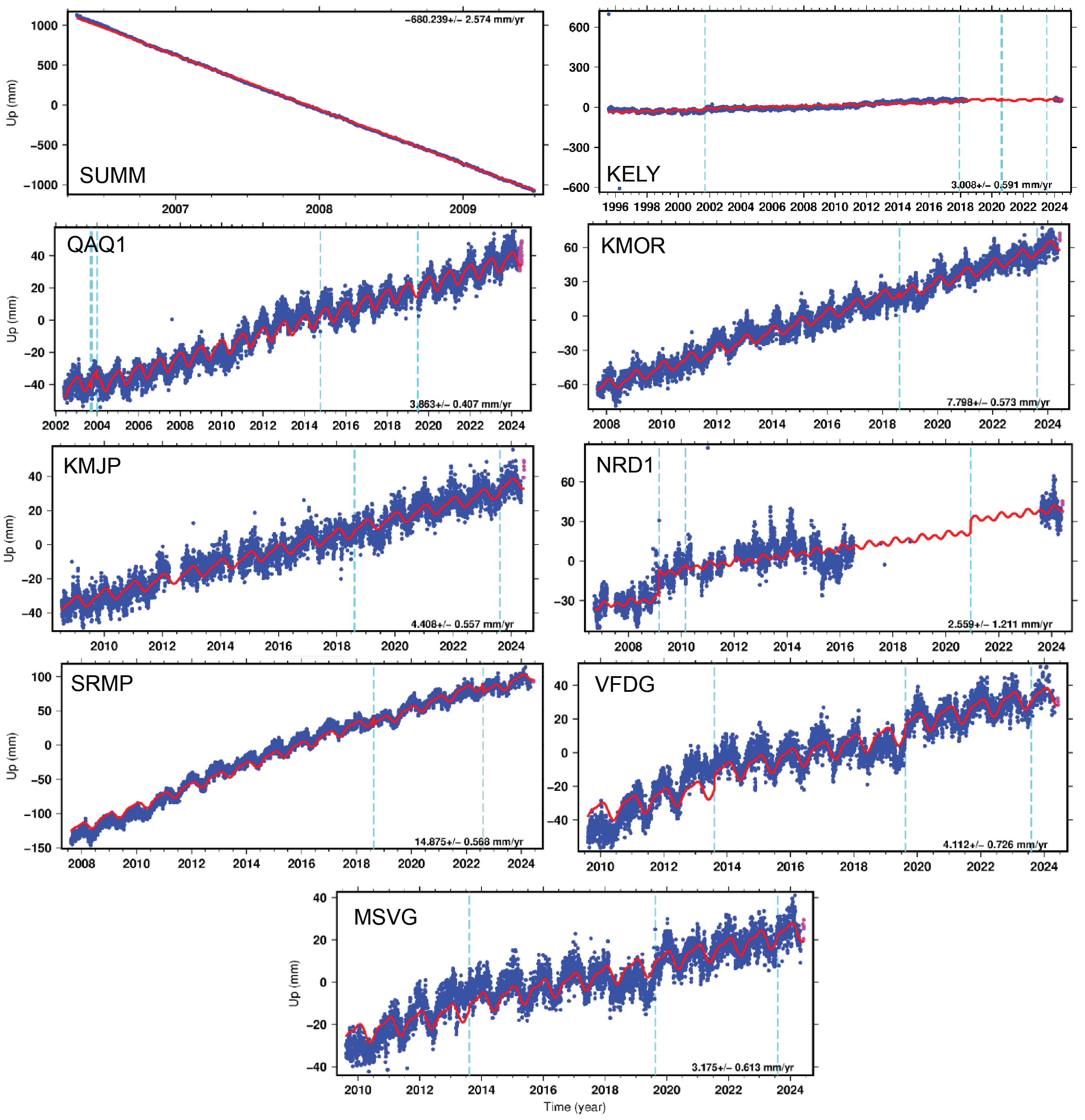
To confirm this, you will use GPS data to monitor glacial change, and its relationship with sea level rise. There are many GPS stations located on the island. We will use those that are continuously recording. GPS data records changes in easterly, northerly, and upward movement. For this exercise, you will only observe the upward or downward movement. Figure 13.12 shows the locations of nine different continuously monitored GPS stations that record data every 5 minutes. Figure 13.13 are time series of the data for these stations.
- Fill in Table 13.3 to summarize velocity at each station using the data in 13.13.
Table 13.3 Summary of Vertical Motions in Greenland Station Rate - Use Figure 13.12 to show the vertical motions using the arrow as scale. This scale can only be used for data less than +/-20 mm/yr.
- Do any of the stations show a decrease in height? Why
- Describe the yearly motion for one station. Why does it increase and decrease?
- Do all areas of Greenland show the same amount of vertical motion? Explain.

13.4 Groundwater, Karst, and Subsidence
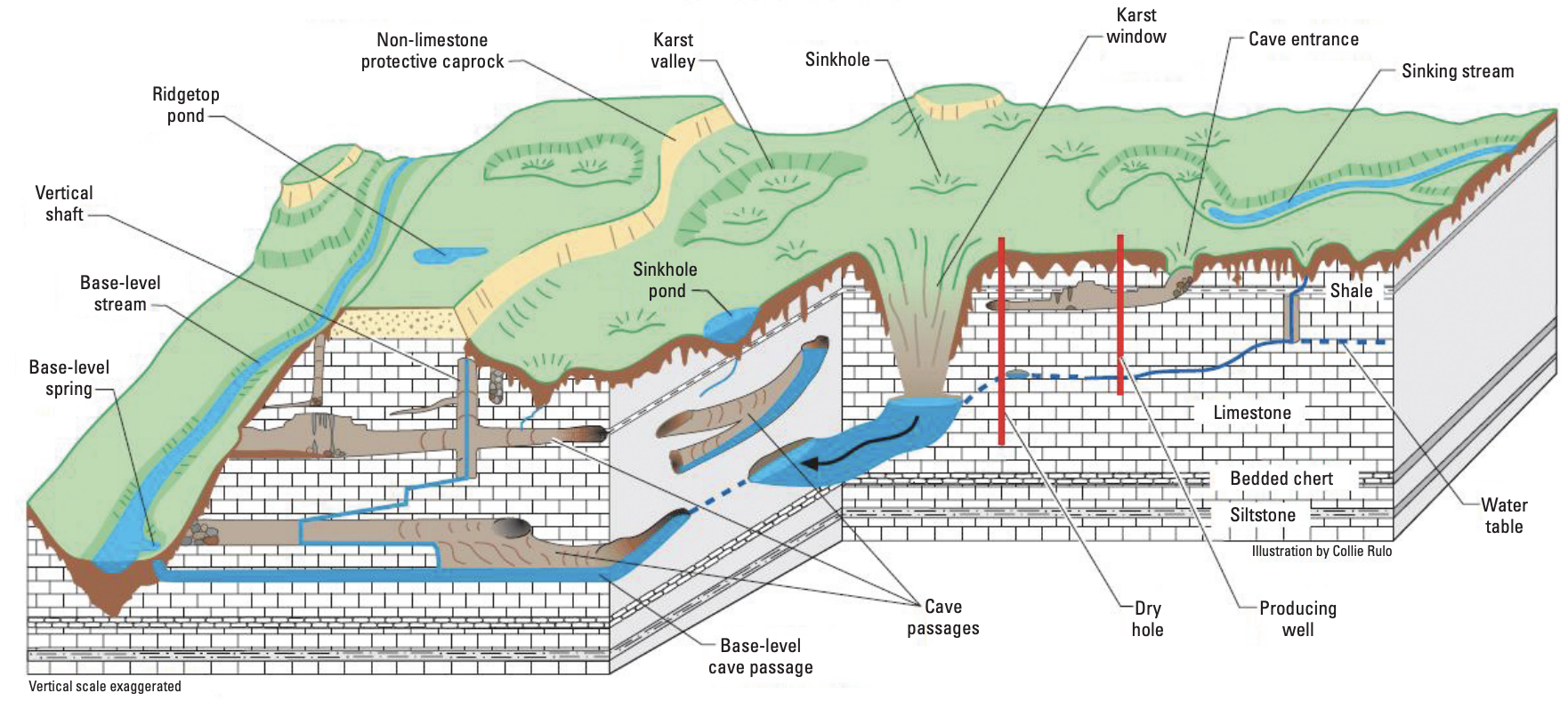
It may not seem like an important part of the landscape, but groundwater flow controls many aspects of geomorphology underground. Caves are a geomorphic feature formed beneath the surface by dissolution of limestone. Limestone at the Earth’s surface can dissolve to form karst topography. Both caves and karst form as carbon dioxide from the atmosphere dissolves in rainwater, making the water slightly acidic. The acidic water widens existing cracks or crevices, which leads to even larger cracks and more water flow and dissolution. In addition to chemical weathering, mechanical erosion occurs as loose rock fragments transported by water erode the sides of the openings.
A critical requirement for the development of karst is water. Without water, there would be no karst or caves. On a global scale, a significant portion (15-20%) of the Earth’s surface is underlain by limestone that has the potential to form karst. Therefore, understanding karst processes is important, particularly where humans interact with this landscape (Figure 13.14). Karst landscapes have features and resources that are not present in non-karst landscapes. Karst aquifers provide the main source of water; for example, 25% of US groundwater comes from karst, such as the Edwards aquifer in central Texas.
Exercise 13.5 – Karst and Sinkholes
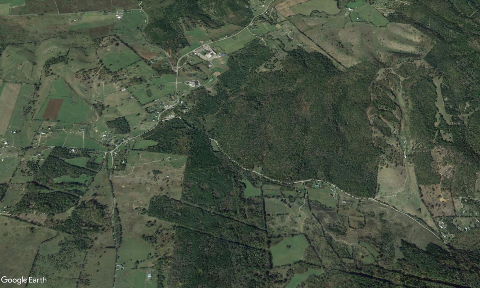
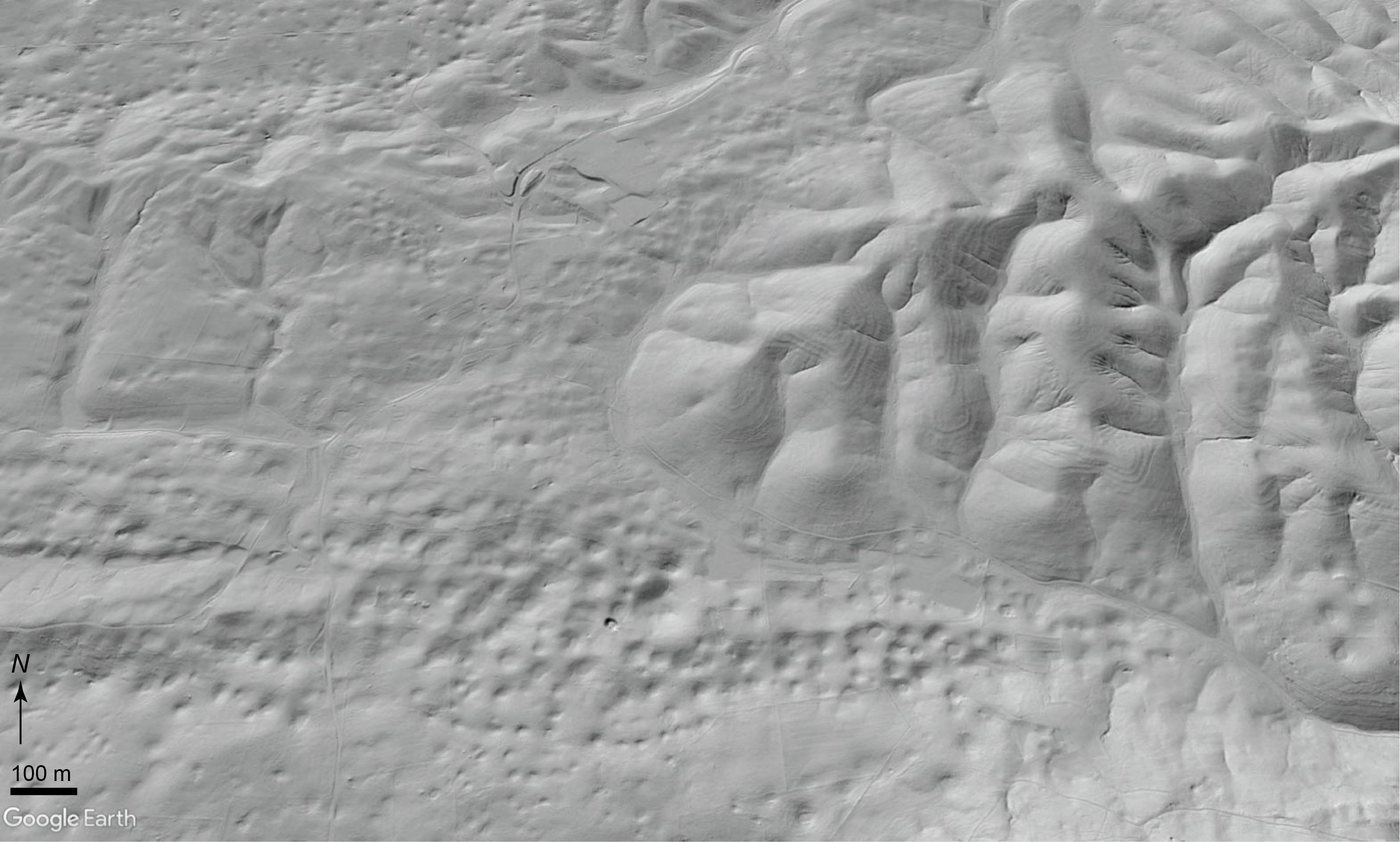
Extensive carbonate occurs in southern Virginia and northern Tennessee. In fact, there is a state park, near Clinchport VA, with a natural tunnel that is over 255 m (838 ft) long that once had a railroad running through it. Compare the satellite image (Figure 13.15) with LiDAR image of the same area (Figure 13.16) for an area east of Natural Tunnel State Park.
- Make observations about the landscape in the tree covered area in the LiDAR.
- Compare this with the farmland surrounding the wooded area. Use Figure 13.15 and name the landforms in the farmland.
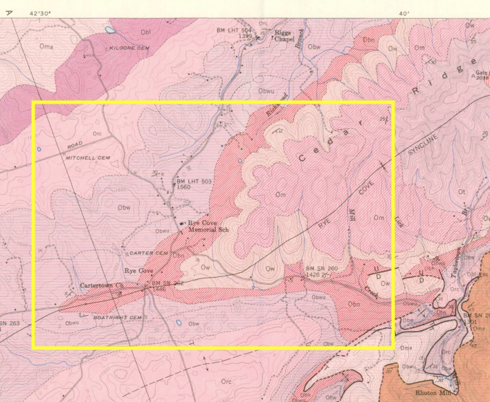
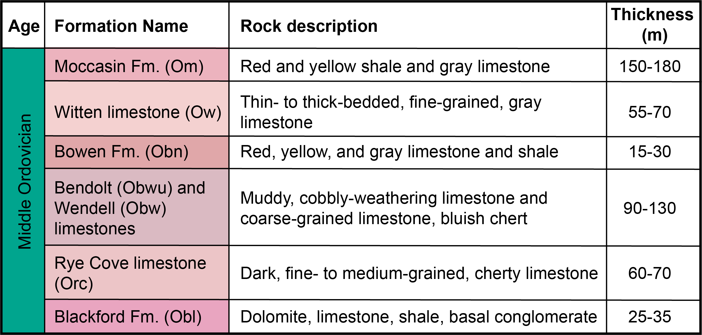
- Use the geologic map and rock descriptions in Figures 13.16 and 13.17 and list the different geologic units in each area.
- Critical thinking: Almost every unit in this area is a type of limestone. Why is some of the area filled with sinkholes and some does not have any karst features?
Both surface water and groundwater play a significant role in landscape development. Groundwater is stored in the open spaces within rocks and within unconsolidated sediments. Porosity is the percentage of open space between grains in a sediment or sedimentary rock. Some volcanic rock has a special type of porosity related to vesicles, and some limestone has extra porosity related to cavities within fossils.
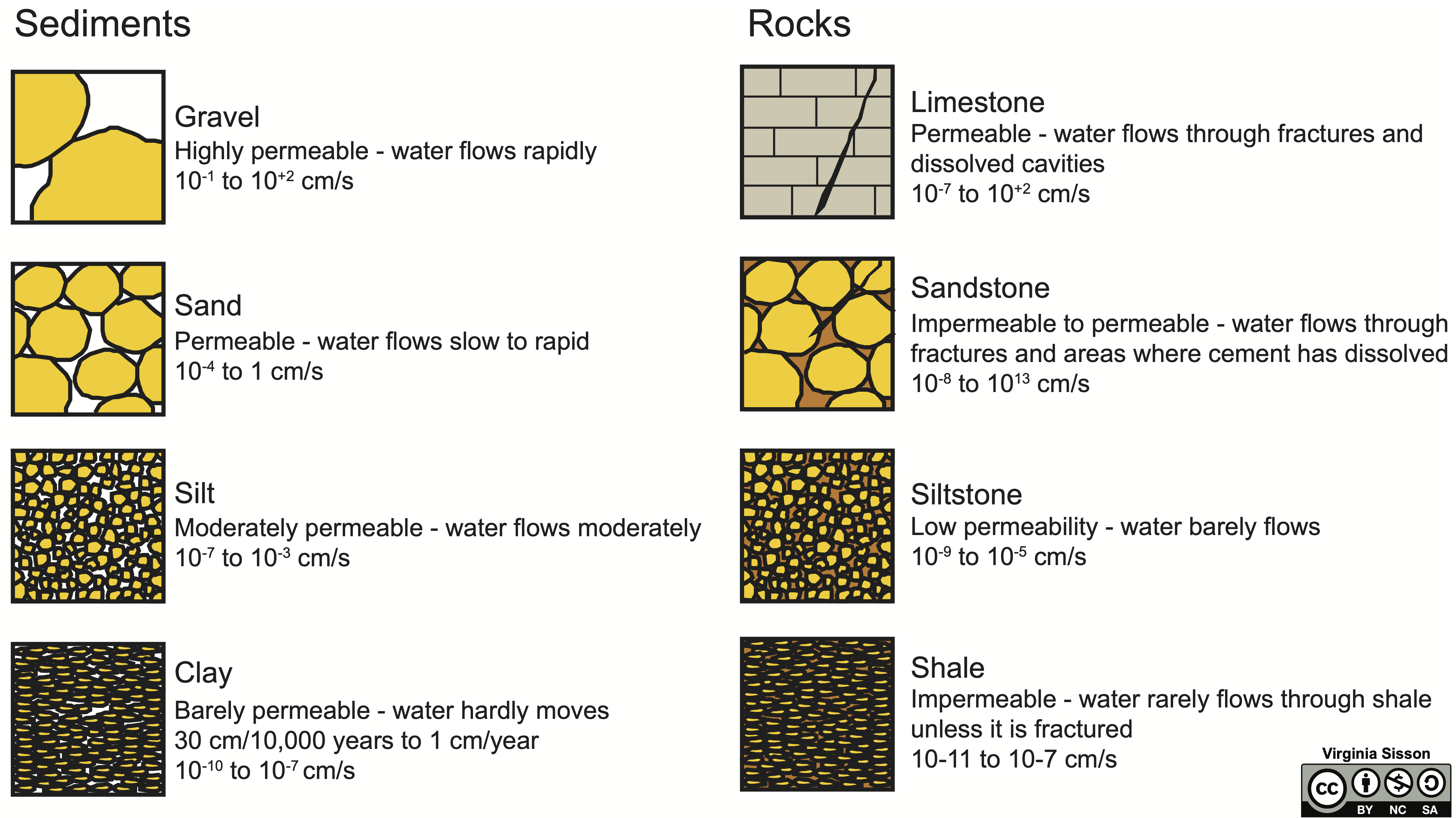
Do you think water can flow through a basalt with lots of vesicles? No, as there is another parameter, permeability, which is the most important variable in groundwater. Permeability describes how easily water can flow through the rock or unconsolidated sediment and how easy it will be to extract the water for our purposes. A permeable material has a greater number of larger, well-connected pores spaces, whereas an impermeable material has fewer, smaller pores that are poorly connected. The characteristic of permeability of a geological material is quantified as the hydraulic conductivity (K) measured as centimeters per second (Figure 13.19).
Exercise 13.6 – Groundwater Flow – Porosity and Permeability
Let’s look at some of the factors that control groundwater flow. Your instructor will provide 3 or 4 containers with sediment with a screened bottom, similar to Figure 13.20.
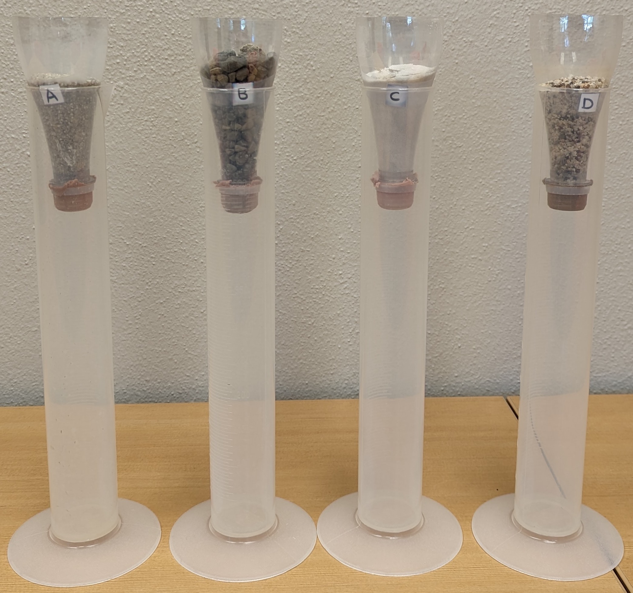
- Pour the same amount of water into each container. Record the time it takes for the water to flow through the sediment. Fill in Table 13.4. Your instructor will determine how many trials you need to do to complete this table.
Table 13.4 – Factors affecting groundwater flow Observation Container 1 Container 2 Container 3 Container 4 Grain size, sorting, and rounding, and sediment type Time elapsed Flow rate (volume/time) Color of water Volume of water retained? - Which sediment transmitted the most water? Which sediment transmitted the least water?
- What properties of these sediments are correlated with good water transmission? Which properties are correlated with flow retardation and water retention?
- Critical thinking: Which of these sediments will provide a clean source of water? Will any of these materials be a good filter for either organic matter or pollutants?
- Now take two samples of porous material – vesicular basalt and coquina and put them across a beaker. Which of these do you think is more permeable?
- Use an eye dropper and pour water over these two samples. Which sample allows water to pour through it? Was your hypothesis correct?
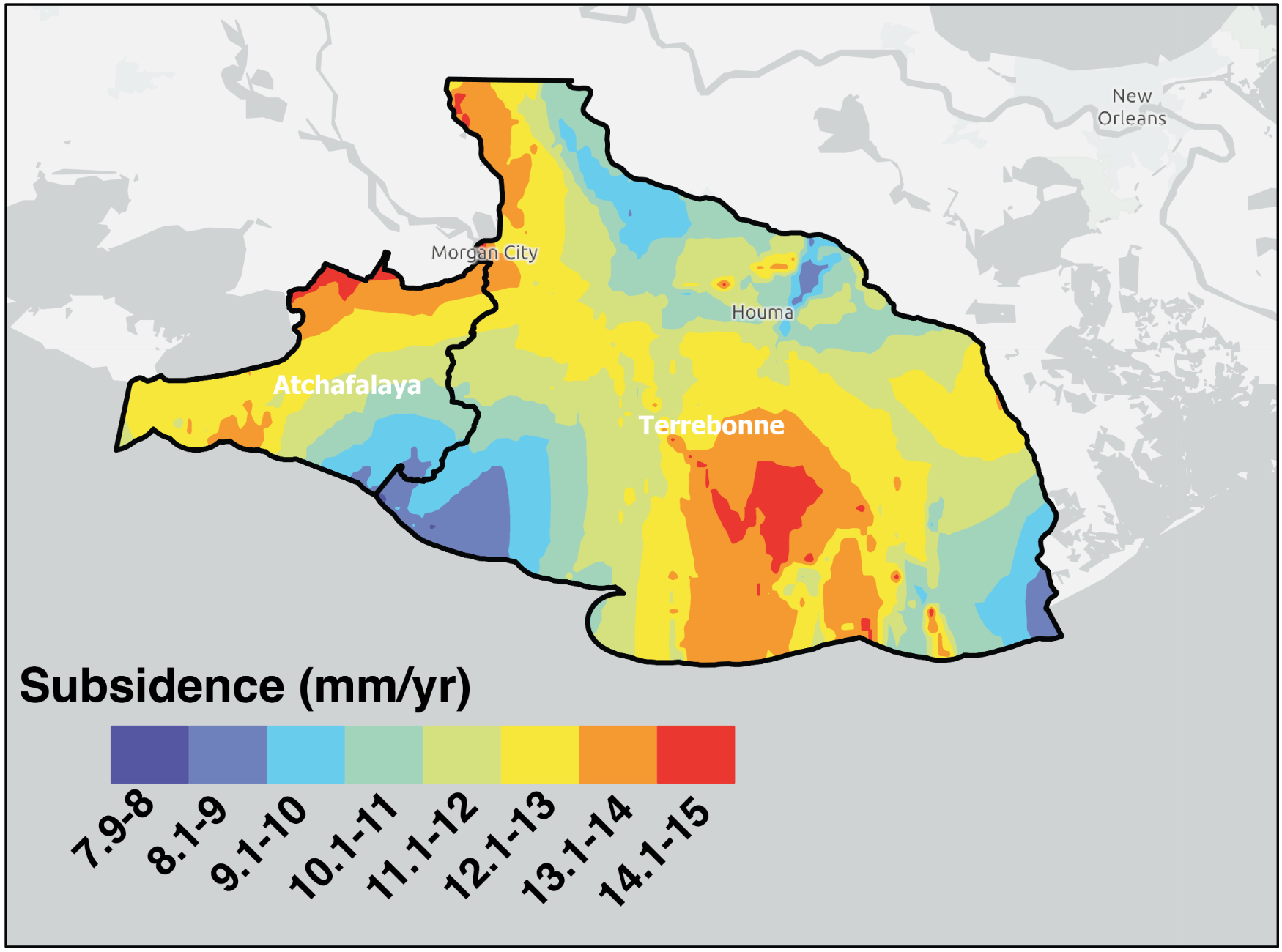
Subsidence may seem like a minor change in the landscape because, in most areas, sinking is negligible. To those living near the coast, it’s a major threat combined with rising sea levels and climate change. Not only will coastal communities be affected, but their water supplies are also susceptible to an influx of saltwater. This problem makes many more vulnerable to sea level changes, such as the Mississippi Delta and America Samoa. This process results in coastal retreat and land loss. In the Mississippi Delta, about 60 km2/year is vanishing. Not only is this important for those who live there, but the Atchafalaya River basin (Figure 13.21) provides flood relief for the Mississippi River, slowing its flow and trapping nutrients and pollution, improving water quality as it flows into the Gulf of Mexico.
Exercise 13.7 – Groundwater Flow – Subsidence
Houstonians started pumping groundwater about 1836, and almost immediately, this began to cause subsidence, with most of the Houston-Galveston area subsiding (sinking) more than 0.3 m (~1 foot). Some areas near Baytown subsided as much as 4 m (~13 feet); an entire subdivision sunk below sea level, and it is now all marsh. In addition, before 1977, Houston aquifers (Chicot, Jasper, and Evangeline) lost ~100 m (300-400 feet). In reaction, the Texas legislature created the Houston-Galveston subsidence district in 1975. One of their first initiatives was to install a network of wells to measure groundwater and subsidence; data collection started in 1977 and continues today. Use this link for recent water well data around Houston. This will show you how water well data is made into a contour map.
- Figure 13.22 shows the water level in wells around Houston TX in 1977. The USGS has shown contour lines relative to sea level (0 feet). You have worked with topographic maps showing relief with contour lines that connect equal points of elevation. You can also use contour lines for other types of data. However, the USGS only contoured part of the data. Finish the contour map.
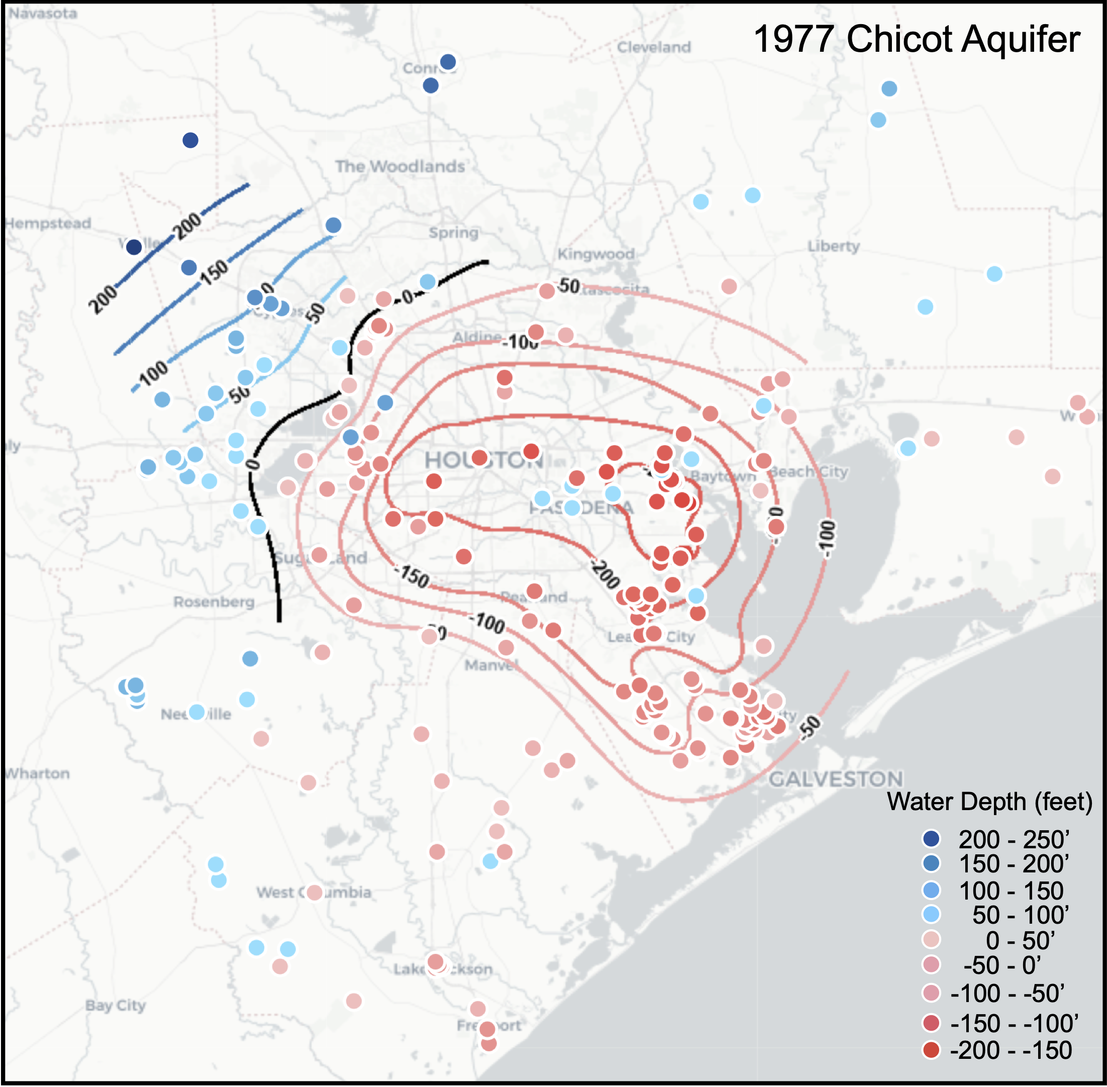
Figure 13.22 – Water well data and contours for Greater Houston area in 1977. Image credit: U.S. Geological Survey Public Domain (note this website is no longer available). - When this data was collected in 1977, Houston was withdrawing ~138 million gallons of water per day, and it is now about pumping only 8 million gallons per day. How has this affected ground water levels? Compare your contour map with the map for the Houston region in 2020 (Figure 13.23).
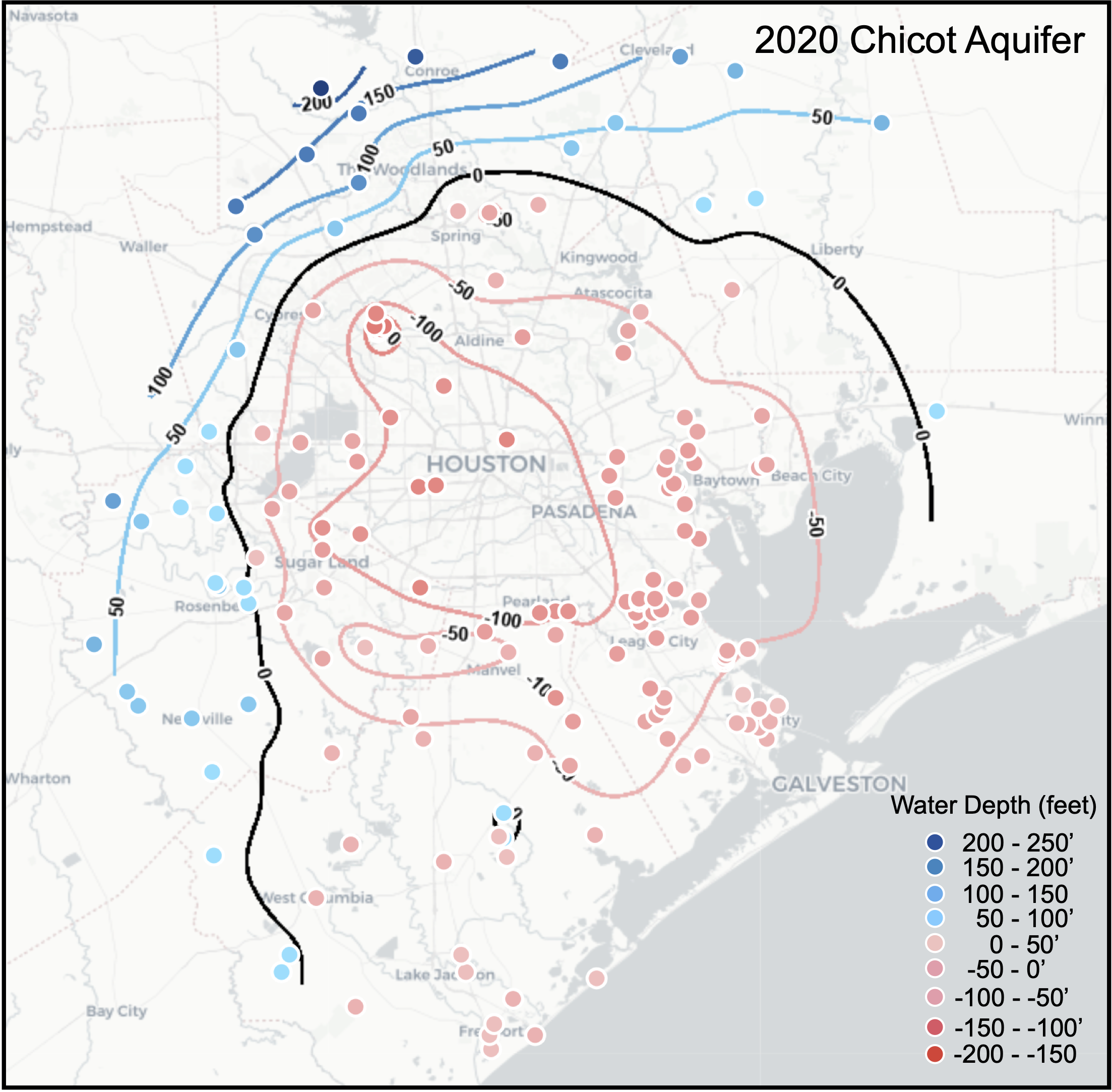
Figure 13.23 – Water well data and contours for Greater Houston area in 2020. Image credit: U.S. Geological Survey Public Domain (note this website is no longer available). - Is the total range of water depths similar? Has the water level increased or decreased from 1977 to 2020?
- How does the sea level contour look in both maps? Has it moved relative to downtown Houston?
- Critical Thinking: Do you think that the water level will keep getting shallower through time? Or will it reach a steady-state value? Explain.
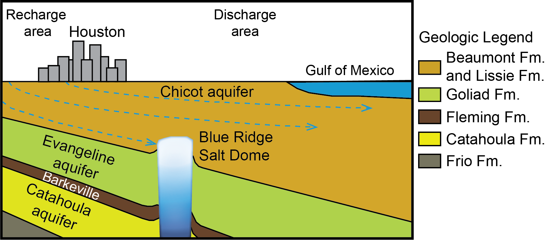
Groundwater exists everywhere there is porosity. However, whether that groundwater is able to flow depends on the permeability. An aquifer is defined as a body of rock or unconsolidated sediment that is permeable. An aquitard, or confining layer, does not allow significant water flow. Figure 13.24 shows a cross-section through the Greater Houston area with various aquifers and confining layers as well as the direction of water flow from where it enters the system in the recharge area to the discharge area.
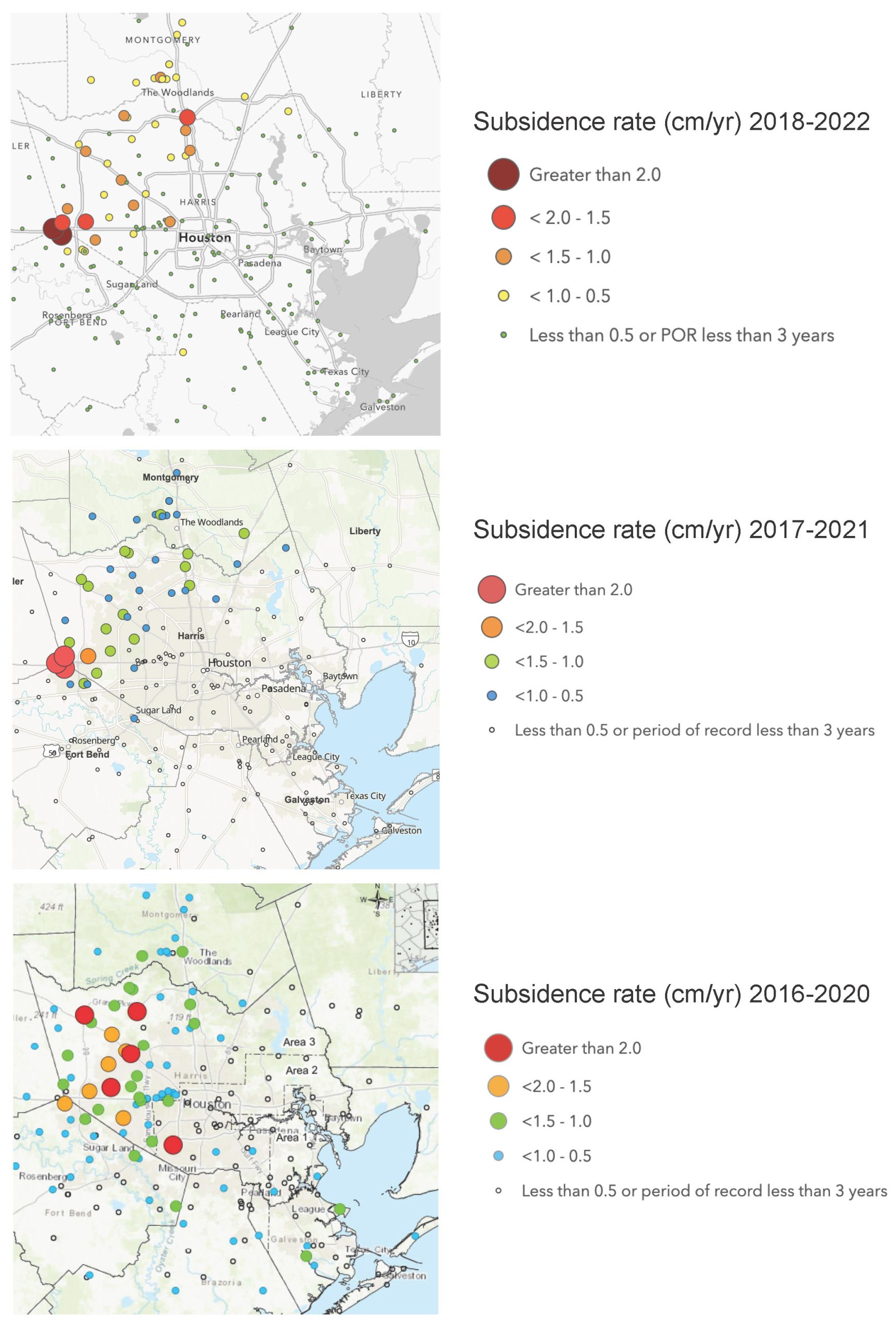
- Next, let’s compare the water level with subsidence rates in these water wells. Contour one of the subsidence maps in Figure 13.25 and compare your results to the rest of the class.
- Where is the most subsidence located?
- Are the patterns from Figure 13.25 similar to the water well contours of Figures 13.22 or 13.23? How are they different?
- Critical thinking: Even without making a contour map, you can see that the amount of subsidence changes with time. Since groundwater withdrawal has been stopped. What other factors could explain the shifts in subsidence rates in this area?
Additional Information
Exercise Contributions
Virgina Sisson, Daniel Hauptvogel, Xiao Yu, and Michael Comas
References
Blewitt, G., W. C. Hammond, and C. Kreemer (2018), Harnessing the GPS data explosion for interdisciplinary science, Eos, 99, https://doi.org/10.1029/2018EO104623.
Brent, W.B., 1963, Geology of the Clinchport quadrangle, Virginia, Virginia Division of Mineral Resources Report of Investigations 5, 47 pp., Map Scale: 1:24,000
Chowdhury, A.H. and M.J. Turco, 2006, Chapter 1, geology of the Gulf coast aquifer, Texas. In R. E. Mace, S. C. Davidson, E. S. Angle, & W. F. Mullican (Eds.), Aquifers of the Gulf Coast of Texas (Vol. 365, pp. 23–50). Austin, Texas: Texas Water Development Board. Report.
Freeze, R.A. and J.A., Cherry, 1979, Groundwater, 604 pp. CC-NC available as pdf
Green, C.A., A.S. Gardner, M. Wood, and J.K. Cuzzone, 2024, Ubiquitous acceleration in Greenland Ice Sheet calving from 1985 to 2022, Nature, 625, 523–528 https://doi.org/10.1038/s41586-023-06863-2
McKee, E.D., 1979, A study of global sand seas, U.S. Geological Survey Professional Paper 1052 https://doi.org/10.3133/pp1052
Taylor, C.J. and E.A. Greene, 2008, Hydrogeologic Characterization and Methods Used in the Investigation of Karst Hydrology, in Field Techniques for Estimating Water Fluxes Between Surface Water and Ground Water Edited by D.O. Rosenberry and J.W. LaBaugh ,U.S. Geological Survey Techniques and Methods 4–D2, 128 pp.
Varugu, B., and C. Jones, 2023. Delta-X: Land Subsidence Rate, Mississippi River Delta (MRD), Louisiana, USA. Oak Ridge National Laboratory Oak Ridge National Laboratory (ORNL) Distributed Active Archive Center (DAAC), Oak Ridge, Tennessee, USA. DOI: 10.3334/ORNLDAAC/2307
the process by which fertile land becomes desert, typically as a result of drought, deforestation, or inappropriate agriculture.
