
Chapter 15: Climate Change
Learning Objectives
The goals of this chapter are to:
- Understand geologic factors in climate change
- Interpret affects of climate change
- Evaluate a possible geologic solution to climate change
15.1 What Affects Earth’s Climate?
Most of us worry about climate change as it may affect our lives and those of future generations. Geological records show that there have been a number of large variations in the Earth’s climate (Table 15.1). These have been caused by many natural factors, including changes in the sun, emissions from volcanoes, plate tectonics, variations in Earth’s orbit, and levels of greenhouse gases such as methane and carbon dioxide. The way these interact with each other makes it complicated. A change in any one of these can lead to enhanced or reduced changes in the others. Also, natural global climate change typically occurs very slowly, over thousands or millions of years.
| Factor | Temperature Rise or Fall | Length of time |
| Plate Tectonics | Rise or fall | Millions years |
| Volcanic Emissions | release CO2 – Rise
release SO2 – Fall |
Days to years |
| Meteorite Impacts | Fall | Decades |
| Earth’s Orbit | Rise or fall | Thousands to millions |
| Sun (sun spots) | No affect | 11 years |
Exercise 15.1 – How Plate Tectonics Affects Climate Change
On long timescales like millions of years, plate tectonics and the position of the continents drastically affect the climate on Earth. Figure 15.1 is a map that shows glacial deposits and geomorphological features that have been identified in the red-shaded regions. These features are about 300 Ma. The black arrows show a general paleo-ice-flow direction based on field data. Though it is believed ice flowed over Antarctica during this time, paleo-ice flow cannot be determined because of the overriding ice present on the continent today. Answer the questions below based on the map and your knowledge of the climate on Earth.

- Are any of these shaded regions known for supporting large, continental glaciers today? Why or why not?
- What do each of the shaded regions have in common geographically?
- Where are ice sheets on Earth located today? Why are they able to last there?
- Do glaciers typically flow from sea to land? How do you explain why glaciers appear to have done this?
- Now that you have thought critically about the map, give a brief explanation for why we see glacial signatures in these regions today.
- Where do you think the paleo-south pole may have been relative to these continents at the time of glaciation? Why? Mark this position on the map with a star.
- Draw a line across the present-day continents showing an estimated position of the equator during this glaciation.
- Do you think these areas may become glaciated again?
- Critical Thinking: How do you think Earth differs when there isn’t a land mass at the poles?
15.2 Glaciers
Did you know that Earth hasn’t always had glaciated polar regions? Earth goes through periods of time when glaciers do and do not exist as its climate changes naturally. In fact, twice in the past, almost every continent was covered in ice during periods geologists call “Snowball Earth.” Our current phase of glaciation began about 34 Ma, and before that, you have to go back to 250 Ma to see the last time ice was present on the planet.
You already looked at landforms left behind by glaciers, now let’s explore the effect of climate on glaciers. You’ll look at alpine glaciers (sometimes called valley glaciers) that originate high up in the mountains, mostly in temperate and polar regions but also in tropical regions in high mountains (e.g. Mount Kilimanjaro in Africa). As these glaciers form, ice builds up where the temperatures are low, then ice begins to flow down-slope with the help of meltwater and sediment, and finally melts when the temperatures are too warm. The flow of alpine glaciers is driven by gravity.
Alpine glaciers grow due to accumulation of snow over time. In the zone of accumulation, the rate of snowfall is greater than the rate of melting. In other words, not all of the snow that falls melts during the following summer. In the zone of ablation, the rate of melting exceeds accumulation. The equilibrium line marks the boundary between the zones of accumulation (above) and ablation (below).
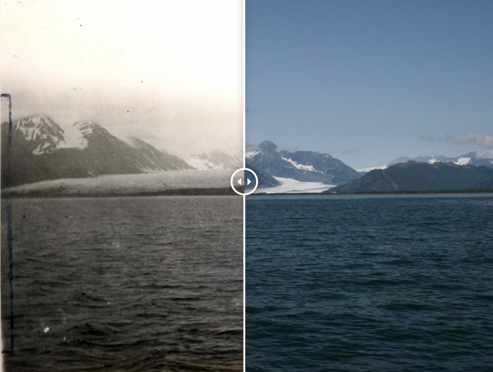
What factors other than gravity control the rate of glacial advance and retreat? Obviously, temperature is important. Also, there must be enough moisture to make snow. Both of these are affected by climate change. News reports have highlighted pictures of receding glaciers such as Figure 15.2. Did you realize that by the year 2100, that over 30% or ~49 trillion metric tons of glacial ice is predicted to melt. Overall, this means ~70% of glaciers will disappear.
Exercise 15.2 – Glacial Advance and Retreat
Visit the glacier simulator to visualize these processes in action. Upon opening the page, familiarize yourself with the parameters you can adjust. If you’re struggling to see the model, uncheck the snowfall box to remove the white haze.
- What happens to the glacier’s length when you turn the average snowfall all the way up?
- What happens when you turn the average snowfall all the way down?
- Reset the model. Hold these parameters steady for about 30 seconds. The small black dots represent sediment sediment transported by the glacier. Where is all the sediment deposited?
- Now, reduce the average snowfall from 3.1 ft to 3.0 ft to make the glacier retreat slightly. Can you still identify the previous position of the ice?
- Turn the sea-level air temperature all the way up. When you increase the average snowfall, what happens to the glacier? Why do you think that is?
- Move the drill tool to the glacier and push on the red button to simulate taking an ice core from the glacier. Try moving it over the zone of accumulation as well as the zone of ablation. What do you notice about the drill hole over time? Why does this happen?
- Check the equilibrium line, which will create a red dashed line at a certain elevation. Use the glacial budget tool (green box) to record the glacial budget at four points along the glacier. Two points should be above the line, and two points should be below. You’ll see three values: accumulation, ablation, and glacial budget. Describe what you observe about the glacial budget and what the equilibrium line means.
- Use the “Advanced” tab. Pause the simulation. Select the glacier length vs. time box and move the popup out of the way. This graph shows how far the glacier will advance or retreat over time. Set the temperature and snowfall parameters for maximum glacial growth and unpause the simulation. When the glacier length reaches 225,000 ft, pause the simulation and set the temperature and snowfall parameters for maximum retreat. Unpause the simulation.
- How many years did it take for the glacier to grow to 225,000 ft? ____________________
- How many years did it take to fully collapse? __________________
- What does this tell you about glacial stability?
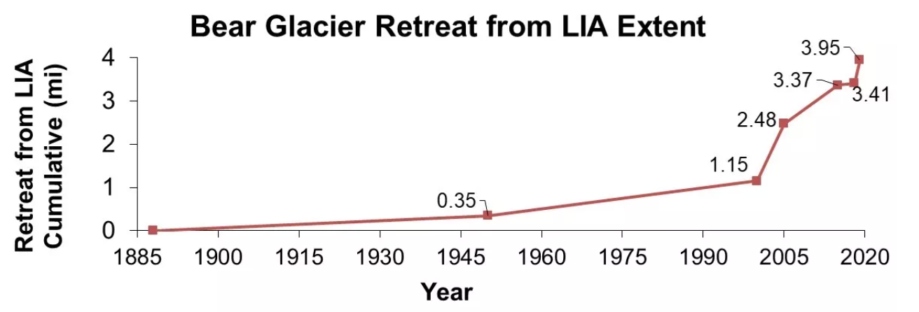
- Look at Figure 15.3 which measures the distance in miles for the retreat of Bear glacier.
- How does this graph compare with theoretical curve you made for question h?
- Do you think climate has been steady or changing in Alaska? Explain.
- Critical thinking: Another factor in this glacial system is the proglacial lake. Occasionally, the beach that dams the lake breaks creating a massive flood (jökalhlaup). This allows ocean water which is both salty and somewhat warmer to flow into this lake and also also experience tides. How will each of these three factors affect glacial retreat?
- How does this graph compare with theoretical curve you made for question h?
15.3 Sea Ice
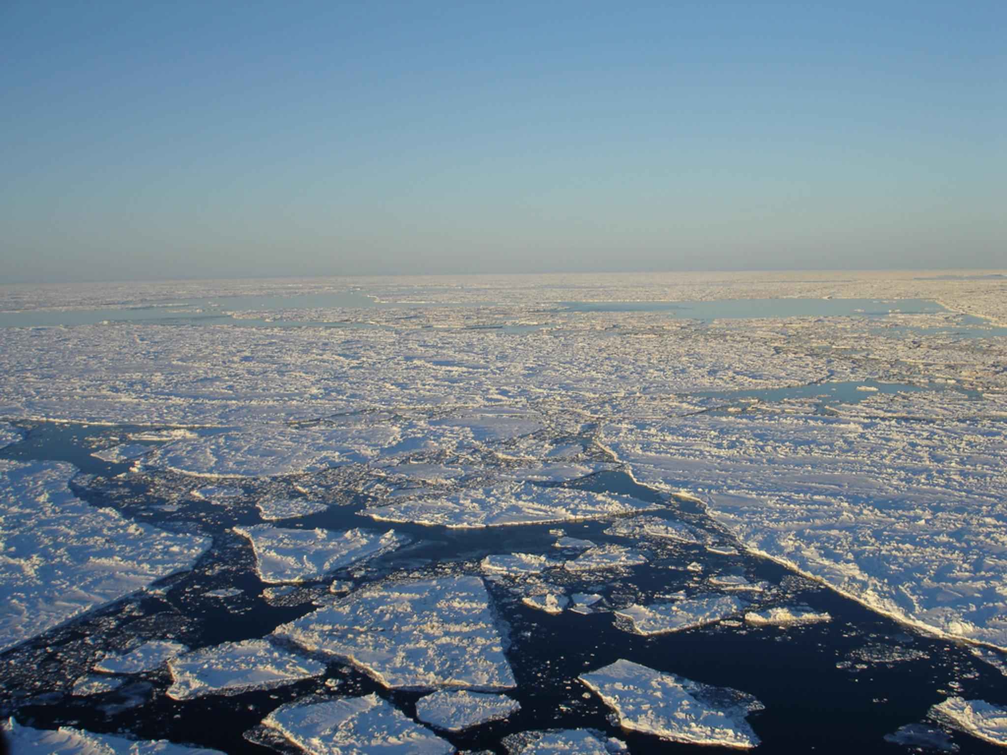
Sea ice is different from glaciers. Sea ice is a thin layer of frozen ocean, (Figure 15.4) and as you know glaciers are ice masses on land. Since sea ice freezes at about -2 oC, it is a sensitive indicator of the ocean temperature. Every year, sea ice forms at each pole; this is a very important event for a number of environmental processes. Sea ice development supports krill populations (the base of the marine food chain), provides passages for certain animals to migrate, increases albedo (the amount of the sun’s energy that is reflected back into space), and helps to drive global ocean circulation. In the Arctic, Russia’s Arctic and Antarctic Research Institute has compiled ice charts since 1933. Today, scientists studying trends ice in the Arctic Sea can rely on a fairly comprehensive record dating back to 1953. To gauge what how much sea ice covered the Arctic Sea before then, scientists use a combination of historical records and proxy measurements such as marine sediment cores. Taken together, these records indicate that the ice covering the Arctic Sea is undergoing an unprecedented decline in the last several centuries.
Exercise 15.3 – Sea Ice
The National Snow and Ice Data Center has tracked the area of sea ice in the Arctic and Antarctic since 1979. Use this data to answer the following questions.
- Hide all data and select the plot for 2023. What can you say about the seasonality of sea ice in the Arctic?
- What is the approximate difference in sea ice extent (in millions of km2) between the peak and trough of 2023?
- Still looking only at the 2023 plot, what can you say about long-term trends in sea ice formation over time?
- Now turn on the 2012 plot as well. With these two data sets, what can you say about trends in sea ice formation over the decade?
- What do you think may have been some possible causes of the anomalously low sea ice in 2012?
- As the site says, 2012 had record low sea ice in the Arctic. Do you think using 2012 data to compare to other years might be biasing our data? Why or why not?
- Turn off the 2012 and 2023 plots. Now select the four decadal averages. What can you say about sea ice trends in the Arctic over the last half-century?
- Critical Thinking: How do you think this may affect the global economy? Which countries do you think may be most closely watching sea ice levels in the Arctic?
15.4 Sea Level
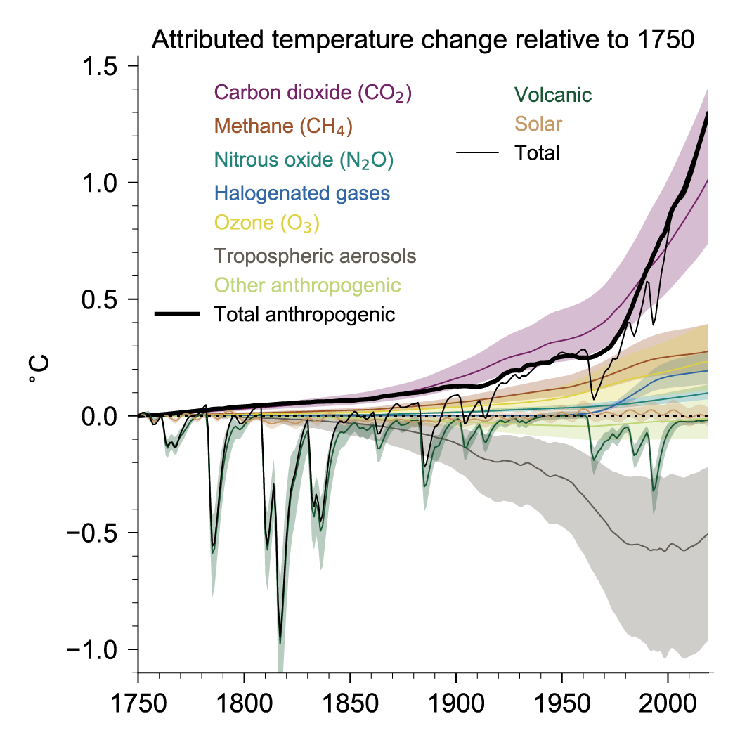
Let’s look at how climate has been changing recently. There are many factors in climate change that are attributed to our atmospheric inputs. Figure 15.5 shows how each different factor has affected climate. This includes natural and manmade changes.
How can we recognize this overall temperature increase in the geologic record and how does this affect geologic processes? Well, sea-level rise is one of the simplest to understand the cause and effects of climate change. Rising sea level is mostly due to a combination of melt water from glaciers and ice sheets and thermal expansion of seawater as it warms. In 2025, global mean sea level was 102.4 millimeters (4 inches) above 1993 levels, making it the highest annual average in the recent record (1993-present).
Exercise 15.3 – Sea-Level Rise and Coastal Erosion
In 1999, the Cape Hatteras Lighthouse in North Carolina was moved from the original position it was built in 1870 (Figure 15.6). Upon its completion, the lighthouse was an estimated 450 meters away from the coastline. Even in 1870, strong storm surges brought seawater to the base of the lighthouse. Following over a century of sea level rise that resulted in even more intense surges, it was determined that to preserve the lighthouse, it should be moved further inland where storms would have less effect on the foundation of the structure. Answer the questions below about the Cape Hatteras Lighthouse and its relationship to sea-level rise.
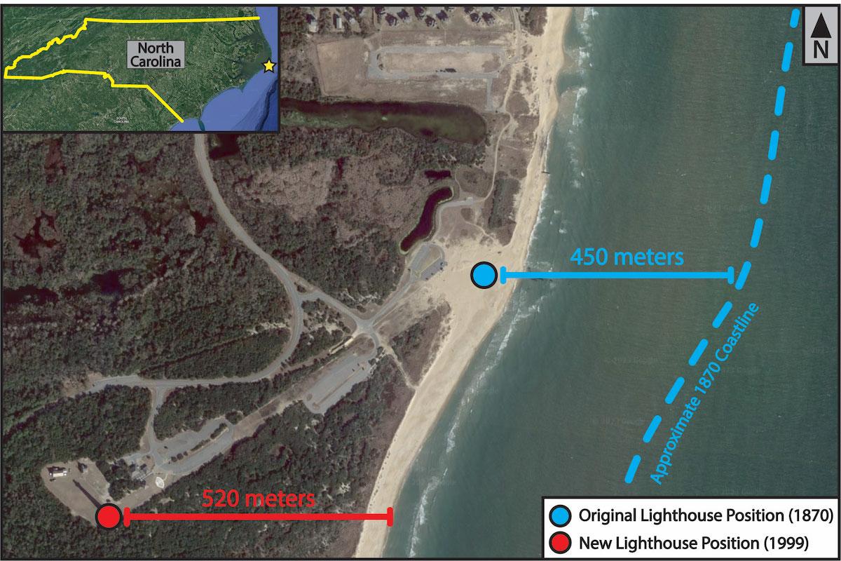
- According to the National Oceanic and Atmospheric Association (NOAA), the pace of sea level rise through most of the 20th century was 1.4 mm/yr. Using this pace, how much has sea level risen since the lighthouse’s construction in 1870?
- If the lighthouse was approximately 450 meters from the coastline when it was built in 1870, and its old position is now ~50 meters from the coast. At what rate (in m/yr) did the shoreline advance onto Hatteras Island?
- Are you surprised by the distance the shoreline encroached compared to the amount of sea level rise? Explain.
- What do your answers say about the slope of the shorefront?
- Do you think this shoreline slope is representative of shorelines around the world? Why or why not?
- Sea-level rise estimates from 2014-2023 put the current pace at 4.77 mm/yr. In 1999, the lighthouse was moved approximately 520 meters inland, how long would it take for the sea to reach this new position of the lighthouse? Assume a constant rate of rise and the same shorefront slope.
- Why do you think the rate of sea level rise has increased so dramatically?
- Critical Thinking: Predictions of future sea-level rise over the coming centuries are highly variable but are expected to increase steadily. What do you think this means for the future of coastal communities and ecosystems?
15.5 Climate Change Mitigation
The term mitigation means to reduce the effects of something. Can your knowledge of geologic processes help solve recent climate change? Yes, is the simple answer. You may have heard the acronym CCUS for Carbon Capture, Utilization, and Storage which are methods and technologies to remove CO2 from the atmosphere, followed by recycling the CO2 for utilization as well as permanent storage options. This is not a new idea as it was first proposed in 1977 and CO2 capture started back in the 1920’s. One major energy company has captured 120 million metric tons of CO2 accounting for approximately 40 percent of all the anthropogenic CO2 that has ever been captured. Most of this captured CO2 is being used for enhanced oil recovery. Some estimate that we need to increase CCUS 70-fold to capture 4 billion tons of CO2 to keep climate change below 2 oC.
What else can be done? Two other proposed solutions are either injecting captured CO2 into the ground or into saline aquifers. To accomplish this, geologic insight is necessary. Deep saline aquifers have the largest identified storage potential, with an estimated storage capacity to store CO2 emissions for at least a century. The captured CO2 can be injected into sedimentary basins below depths where the temperature exceeds 31.1 oC. Why? Well, it relies on two fundamental chemical properties – supercritical fluids and immiscibility. Supercritical fluids are neither a gas or liquid; for CO2 this occurs at temperatures above 31.1 oC. The other is immiscibility, which is like oil and water in salad dressing – they don’t mix. The same is true for salty water and CO2 when it is a supercritical fluid. Also, for this exercise, you need to understand aquifers, so you may want to review your results for exercises 13.6 and 13.7.
Exercise 15.4 – Carbon Capture
First let’s explore, the relationship between permeability and immiscible liquids. Since your lab classroom is below 31.1 oC, we can’t use CO2 for this demonstration. Your TA will hand out demo bottles with glass marbles that represent sand grains and one filled with one liquid and the other filled with two immiscible liquids of different density. Your bottle may have either oil and water or water and alcohol. Food coloring has been added to make it easier to see the water. Turn these upside down and observe what happens. Then flip them back upside right.
- Bottle A – Record your observations:
- Bottle B – Record your observations:
- Aquitards or seals are natural barriers to fluid flow. In sedimentary rocks, these are impermeable rocks such as shale. Which one of these two bottles has an aquitard? Explain.
Modeling carbon storage in western Canada yields a conservative estimate that this area has the capacity to store 56 gigatons of CO2, but could be as high as 360 gigatons (Hares et al., 2022). To put this number into perspective, the conservative estimate of 56 gigatons, would be ~10-13% of the current CO2 budget. To help you visualize this, it is equivalent to all the CO2 emitted by producing plastic for the next 25 years. Still don’t have a good grasp of how much this is equivalent to, the amount of CO2 emitted to make one single polyester shirt is somewhere between 3.8 and 7.1 kilograms, which is a lot shirts worth of CO2 that could be stored underground in western Canada!
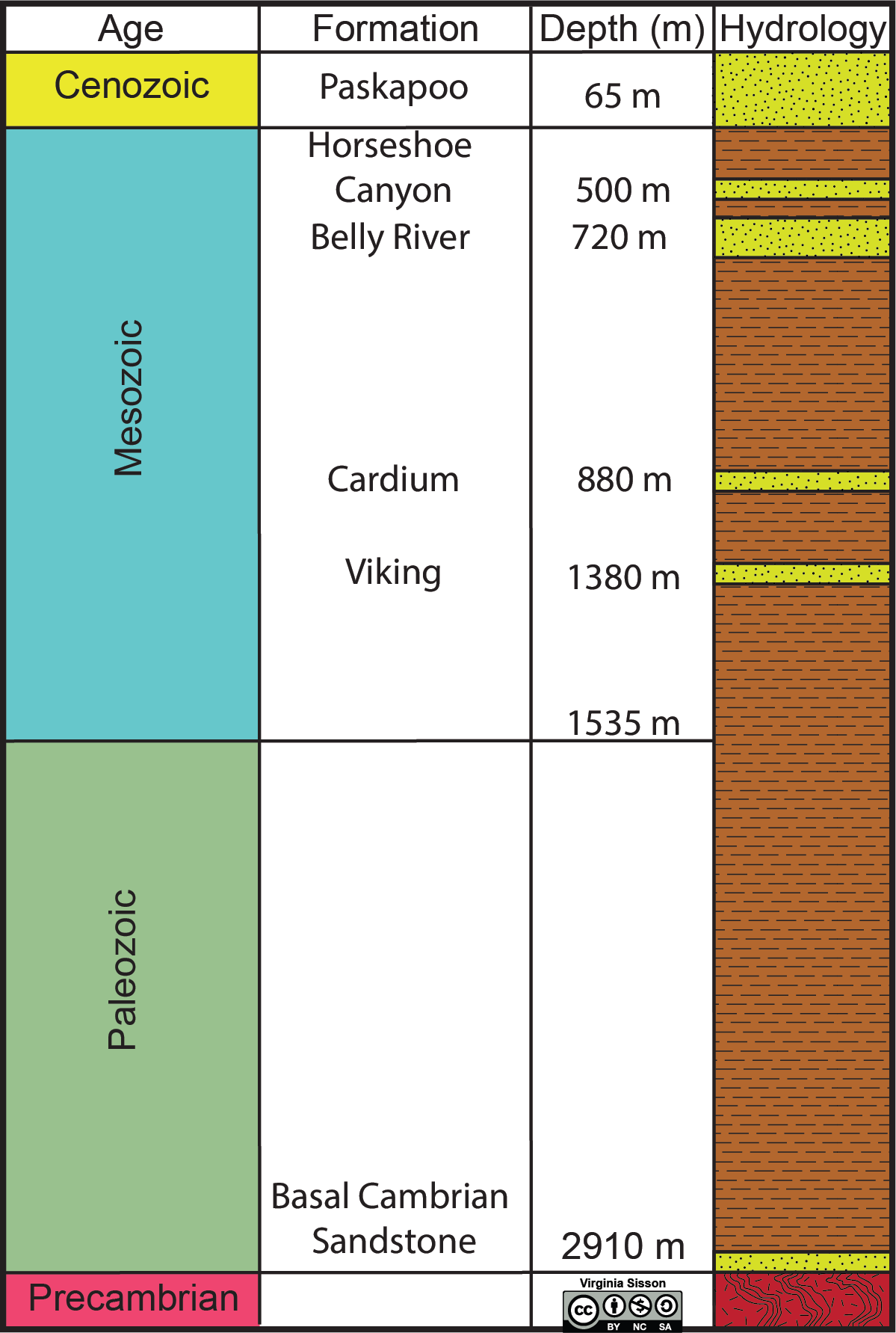
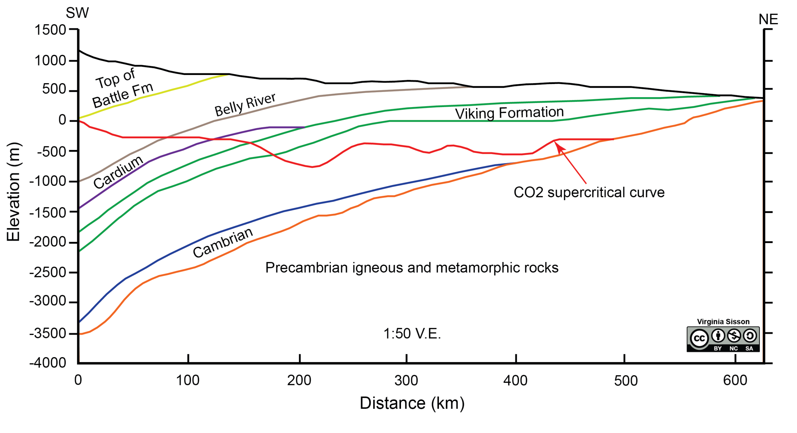
Now let’s look at some of the local geology to figure out where to they propose to put all of this CO2. It needs to go into an aquifer that is beneath the supercritical temperature for CO2. Look at Figures 15.7 and 15.8 to help decide where all of this CO2 will be injected into a saline aquifer. Geoscientists use different conventions for stratigraphic versus cross-section data. Stratigraphic data is given the depth from the surface whereas the cross-section gives elevation above and below sea level.
- First convert the elevation for the supercritical point for CO2 into depth. What is the shallowest depth in a well that will be above the supercritical point? What is the deepest depth?
- Some of these aquifers are too shallow as they would not have supercritical CO2. Which aquifers are too shallow and are above the supercritical point for CO2 storage?
- Which of the other aquifers do you think would be good for for CO2 storage? Of these, predict which would be the best target and why?
- Currently, there are two operational sites in western Canada that are injecting CO2 into the Cambrian aquifers. First is Aquistore in Saskatchewan, injecting CO2 produced at the SaskPower carbon capture facility down to a depth of 3.4 km. The second is Shell Quest in Alberta, which captures CO2 produced from converting tar sands into gas, transporting the CO2 for 65 km and then injecting it to a depth of ~2.0 km. Considering these two projects, which do you think is more successful?
- Critical thinking: What additional information would you need to predict which would be the best aquifer for CO2 storage?
Additional Information
Exercise Contributions
Michael Comas, Virginia Sisson, and Daniel Hauptvogel
References
Hares, R., S. McCoy, D.B. Layzell, 2022, Review of Carbon Dioxide Storage Potential in Western Canada: Blue Hydrogen Roadmap to 2050, Transition Accelerator Reports, 4, 6, 1-42
Intergovernmental Panel on Climate Change (IPCC). The Earth’s Energy Budget, Climate Feedbacks and Climate Sensitivity. In: Climate Change 2021 – The Physical Science Basis: Working Group I Contribution to the Sixth Assessment Report of the Intergovernmental Panel on Climate Change. Cambridge University Press; 2023:923-1054. doi: 10.1017/9781009157896.009.
