
Chapter 9: Earthquakes
Seismic Waves, Hazards, and their Distribution
Learning Objectives
The goals of this chapter are to:
- Understand earthquakes and their associated hazards
- Use seismic waves to locate earthquakes
- Evaluate earthquakes related to induced seismicity
9.1 What are Earthquakes?
An earthquake is the shaking caused by breaking and movement of rocks beneath Earth’s surface. Why does the Earth move? When it is under stress, it deforms, then breaks and two sides slide past each other. Because most rock is strong (unlike loose sand), it can withstand a significant amount of stress without breaking. But every rock will rupture (break) once that limit is reached. For the case of rocks within the Earth, the rock breaks at depth and there is displacement along the rupture surface. This release of built-up elastic energy radiates away as seismic waves. The magnitude of the earthquake depends on the extent of the area that breaks (the area of the rupture surface) and the average amount of displacement (sliding).
In Chapter 2 you discovered that earthquakes occur near plate boundaries. Both divergent and transform boundaries have shallow earthquakes, whereas subduction zones can have deep earthquakes. But not all earthquakes occur along plate boundaries (Figure 9.1).
Exercise 9.1 – Observing Earthquake Hazard
Earthquakes pose a significant risk to the destruction of infrastructure and buildings and loss of life. Figure 9.1 is an earthquake hazard map of the U.S. Answer the questions below.
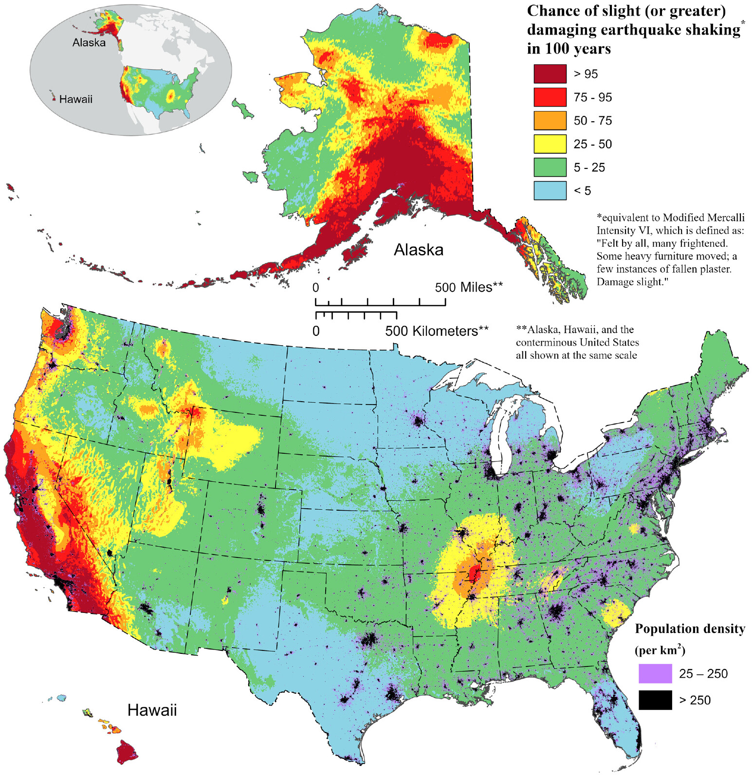
- Explain what the colors on Figure 9.1 mean.
- Which parts of the U.S. have a high earthquake hazard?
- Which parts of the U.S. have a low earthquake hazard?
- Why are earthquake hazards high on the west coast of the U.S.?
- Do any locations of high earthquake-shaking hazards not correspond to any plate boundaries? Can you come up with an explanation for these areas?
- Critical Thinking: Will places on the map that have the same color have the same level of damage if an earthquake occurs?
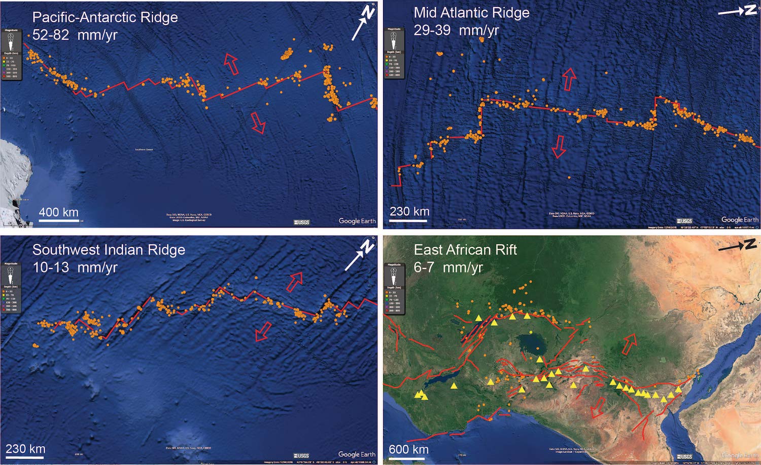
Exercise 9.2 – Comparing Earthquakes at Divergent Plate Boundaries
Divergent plate boundaries occur in both oceanic and continental crust. In oceanic plate boundaries (mid-ocean ridges), numerous transform faults offset these ridges. The location of earthquakes along these divergent boundaries is controlled by whether or not the divergent boundary and/or transform breaks due to brittle deformation. The brittle behavior of rocks is partly a function of temperature and pressure. Typically, only shallow and cool rocks will break. So, you can look at the patterns of earthquakes to determine if a mid-ocean ridge is hot or cool. Why is this important? Well, life and mineral resources are both sensitive to the thermal conditions at ridge crests.
- Look at the patterns of the earthquakes for four different divergent zones (Figure 9.2). Describe the earthquake distributions in the oceanic (A-C) and continental rifts.
- Oceanic
- Continental
- Oceanic
- For images A-C, are most earthquakes located on the spreading ridges, transforms, or both? Also, note if there are earthquakes located off the spreading ridge. Describe where the earthquakes are in images A-C.
- Is there a relationship between the spreading rate and earthquake distribution? Discuss this as a class to explain what you observe.
- An important feature of mid-ocean ridges is black smokers (hydrothermal vents). These form near or on spreading ridges in response to the thermal structure of a ridge, sea water interaction, and fracturing. They are sites for both mineral deposition and deep sea life. Which of these spreading ridges would you predict to have more black smokers? Why?
- Look at the distribution of earthquakes and volcanos in the East African rift zone. Do these occur in the same region? Explain your observations.
- Continental rifts occur in thick continental crust that is hard to break. Would you predict that there would be deeper earthquakes in continental rift zones? Do your observations support or disprove your hypothesis?
- Critical Thinking: The East African rift valley is home to most of the African large mammals as well as where hominid evolution began. What features of this rift are important for biologic and evolutionary activity?
9.2 Seismic Waves
As you can imagine, technology does not exist to travel into all of Earth’s layers. Geoscientists learn a great deal about Earth’s structure through seismic waves. Seismic waves are vibrations in the Earth that transmit energy and occur during earthquakes, volcanic eruptions, and even man-made explosions and nuclear blasts.
Exercise 9.3 – Analogs for Seismic Wave Motion
When an earthquake occurs, seismic waves are released outward from the hypocenter (the location inside the Earth where the earthquake occurred). These waves have different characteristics, including their motion and velocity.
- Using a slinky (can be either metal or plastic), hold one end and have a partner hold the other. Stretch the slinky to at least 8″. If you have a super slinky, you can go even further. Quickly push the slinky forward on your end and immediately pull back. Describe what happens.
- With the same setup, quickly move your end of the slinky up, down, and back to the middle. Describe what you see.
- Discuss with your instructor what these models represent.
- If you shorten or lengthen the slinky, what is the result?
- Does it make a difference if the slinky is metal or plastic? Why? ___________________
- Seismologists like to know the relationship between wavelength, frequency and amplitude of waves. Set up an experiment to demonstrate these with your slinky or with several slinkies.
You can picture seismic waves moving through the Earth as circular waves similar to what happens when a stone is thrown into a pond, but more complex. Seismic waves can be distinguished by a number of properties including the speed the waves travel, the direction that the waves move particles as they pass by, and where they don’t propagate. In the previous exercise with a slinky, could you measure the wave speed? Typical seismic wave speeds are 330 m/s in air, 1450 m/s in water and about 5000 m/s in granite. The precise speed that a seismic wave travels through the Earth depends on several factors, most important is the composition of the rock.
Exercise 9.4 – Seismic Wave Velocity
When an earthquake occurs, seismic waves are released outward from the hypocenter (the location inside the earth where the earthquake occurred). These waves have different characteristics, including their motion and velocity.
- Imagine two cars on a highway are driving right next to each other. Car 1 is traveling at 60 mph, and Car 2 is traveling at 70 mph. Both will maintain their speed. How far apart are the cars after 1 hour? ____________________
- After 2 hours? ____________________
- After 5 hours? ____________________
- How many hours must pass for the cars to be 100 miles apart? ____________________
- If the time is 5:30 p.m. and the cars are 75 miles apart, at what time did they start moving? ____________________
- Seismic waves work the same way. P-waves and S-waves travel at different velocities away from the earthquake focus (Figure 9.3). Which wave travels faster? ____________________
- How long does it take a P-wave to travel 1,000 km? ____________________
- How long does it take an S-wave to travel 1,000 km? ____________________
- You can use the difference in travel time to determine how far away an earthquake occurred. If the travel time difference between a P-wave and S-wave is 1 minute, how far away was the earthquake? ____________________
- Critical Thinking: Does this tell you the exact location of the earthquake? Why or why not?

The measurement for how powerful an earthquake is is called its magnitude. The magnitude can vary from place to place based on distance, type of surface material, and other factors. You may have heard about the Richter scale (MR) for measuring magnitude, which is based on the amplitude of the seismic waves, but in practice it’s not commonly used anymore. The Moment Magnitude (MW) is more accurate, especially with more power earthquakes. It’s based on the strength of the rock along the fault, the area of the fault that slipped, and the distance the fault moved. Thus, stronger rock material, or a larger area, or more movement in an earthquake will all contribute to produce a larger magnitude.
9.3 Locating Earthquakes
Since earthquakes all over the world, how do we determine where they occur? Sometimes they occur in the middle of the ocean or in remote areas where no one lives. Is this like the age old question that if a tree falls in the woods, does it make a sound? Even if there’s no person or other animal around to hear the tree falling and crashing, a recorder with a microphone could certainly record those vibrations—as sound. The same is true for earthquakes. Geoscientists have set up earthquake monitoring stations using seismometers around the world to record earthquake waves. These are set-up on global, national and regional scales. For example, the San Francisco Bay region has over 550 local monitoring stations while the Global Seismographic Network only has 152.
Do you want to set up your own earthquake monitoring station? You can with your smart phone as these have motion sensors to determine whether your phone is stationary or falling out of your hand. These include Seismograph, iSeismo, and VibrationMeter. In addition, there are now apps to help alert you if you live in an earthquake prone area, such as MyShake and Earthquake.
Exercise 9.5 – Locating an Earthquake
The location of earthquakes can be found by triangulating the origin of seismic waves. Figures 9.4 – 9.6 contain three-component seismograms for three different locations. The three components represent different directions of motion: Up-Down (vertical), North-South, and East-West.
- On Figures, mark the arrival of the first P waves, S waves, and surface waves.
- Determine the arrival times of P and S waves at each station (Figures 9.3 – 9.5). Be as exact as possible and record the times in Table 9.1.
Table 9.1 – Seismic wave data to locate an earthquake Seismic Station Location P wave arrival time S wave arrival time S-P time (mm:ss) Distance (km) Tuscon, AZ Corvallis, OR Cathedral Caves, MO - Determine the amount of time between the arrival of P and S waves at each station. Record the time difference in Table 9.1.
- Now that you know the difference in arrival times, you can tell how far away the earthquake was from each station. Use Figure 9.3 and find the chunk of time between the two curves. Record the distance in Table 9.1.
- Now, you’re going to triangulate the location of the earthquake. You can do this one of two ways:
- Head to the Iris triangulation webpage. Click “+ Station” and input the latitude and longitude of each station and the distance of the epicenter you determined. Look at the bottom of the page to edit this data. This will create a colored circle around each station that has a radius equal to the distance you entered. If you select this, show your instructor the map you made on the Iris webpage, then mark the earthquake’s epicenter on Figure 9.7.
- Plot the three circles of your measured distance for each station using a compass on Figure 9.7. For both ways, where the three circles intersect (or come close to intersecting) is the location of the earthquake.
- Is this earthquake located near a plate boundary? If so, what type of plate boundary is nearby?
- How could you determine a more precise location?


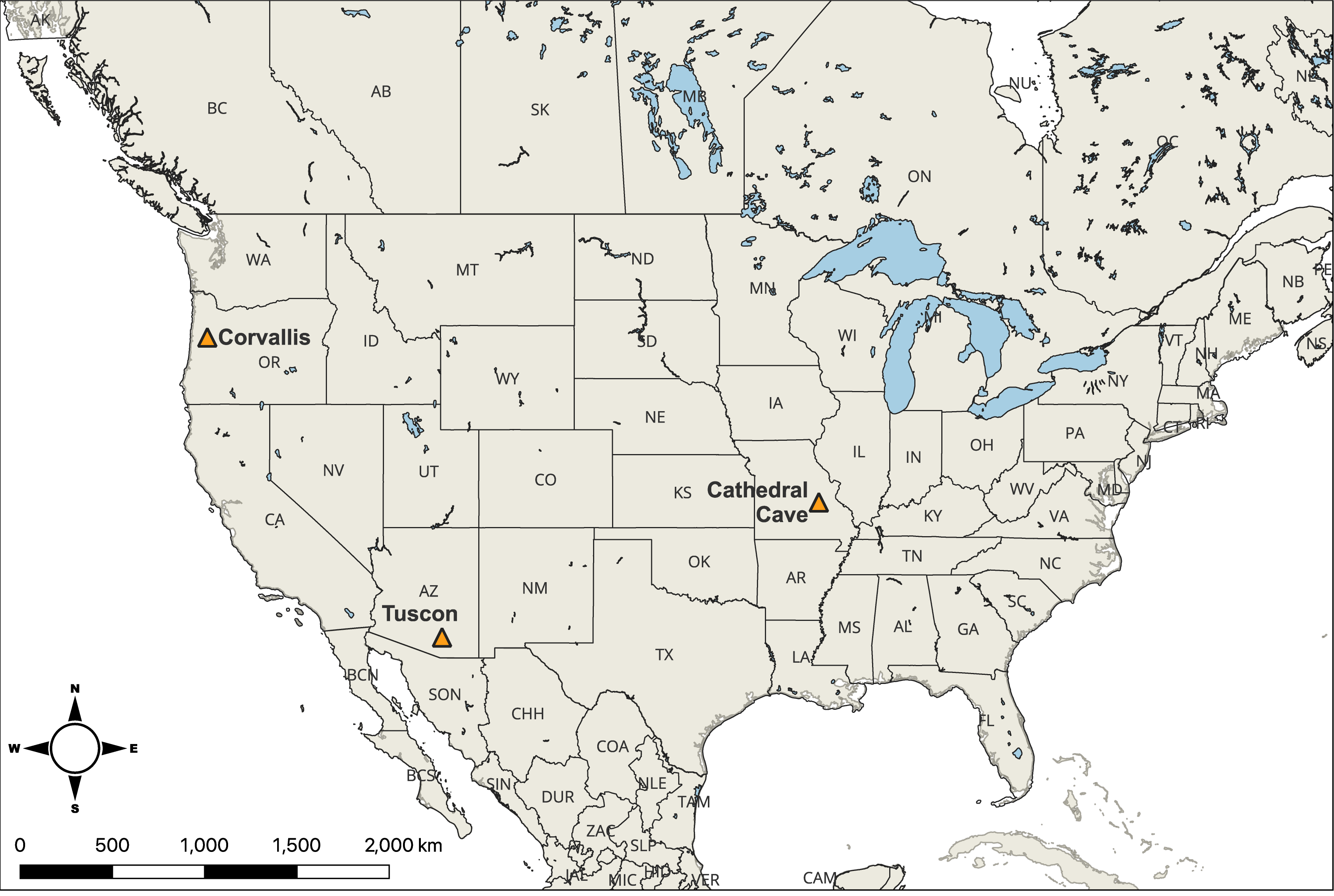
This exercise is adapted from IRIS/SAGE.
9.4 Induced Seismicity
Induced seismicity is typically earthquakes and tremors that are caused by human activity that alters the stresses and strains on Earth’s crust. The first case of induced seismicity occurred in 1932 in Algeria’s Oued Fodda Dam. Most induced seismicity is of a low magnitude. Injecting fluid underground can induce earthquakes, a fact that was established decades ago. Injection increases the fluid pressure within the Earth, creating an area more likely to fail in an earthquake. When injected with fluids, even faults that have not moved in historical times can be made to slip and cause an earthquake.
Why inject fluid underground? Several reasons are wastewater disposal, hydraulic fracturing and enhanced oil recovery. Within the United States, each of these activities has induced earthquakes in the past few years. These are regulated under the Safe Drinking Water Act with standards set by the U.S. Environmental Protection Agency. Other purposes for injecting fluid underground include enhanced geothermal systems and geologic carbon sequestration.
Exercise 9.6 – Fracking and Earthquakes
Since 2001, oil and gas have been extracted from shale, but shale is not a permeable rock, so fluids can’t pass through it. Geologists can increase the permeability of shale so that oil and gas can flow and be extracted. This is done by hydraulic fracturing (“fracking”). During fracking, fluids are pumped into a well at high pressure to open and widen cracks in the shale, allowing the oil and gas to flow easier. This process causes small earthquakes (magnitudes smaller than 1), but large ones do occur with the largest induced earthquake being a M4 in Texas.
In addition, wastewater (a by-product of fracking) is frequently disposed of by injection into deep wells. The injection of wastewater into the subsurface can also cause earthquakes that are large enough to be damaging. Wastewater is injected deep underground, far below groundwater or drinking water aquifers. The largest earthquake known to be induced by wastewater disposal was a M5.8 earthquake that occurred near Pawnee, Oklahoma, in 2016.
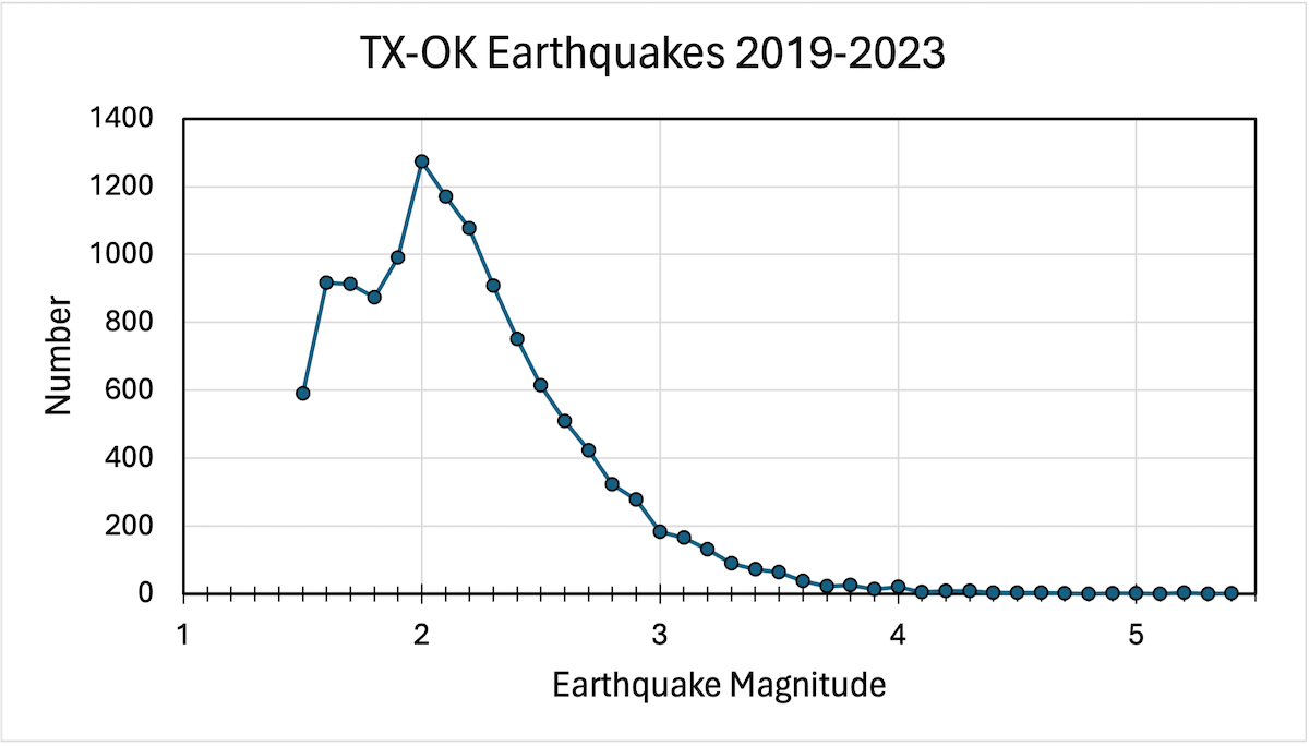
Both fracking and wastewater disposal processes have affected Texas, Oklahoma, and New Mexico. Figure 9.8 shows the distribution of all earthquakes for two five-year periods 1997-2001 and 2019-2023, and Figure 9.8 shows the frequency of earthquake magnitude from 2019-2023.
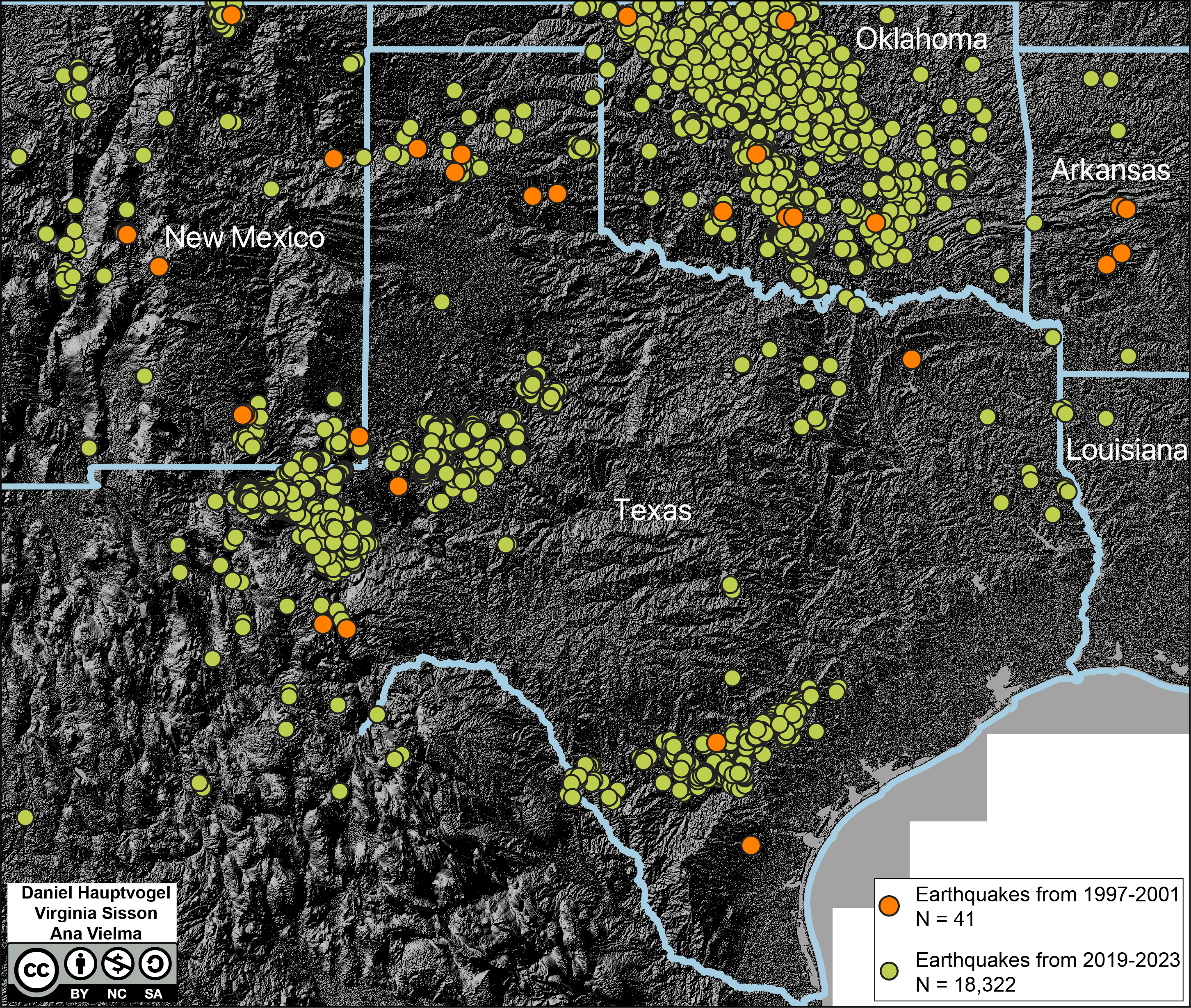
- Use the 1997-2001 data from Figure 9.8 to determine the natural seismicity and where it occurred in this region. Do the earthquakes cluster in distinct areas? If so, where are these located?
- Look at Texas in Figure 9.8, are the orange-colored earthquakes associated with any specific rocks? Open the interactive map of the geology of Texas and look at the regional trends and rock types; look to see what type of sedimentary rocks are there.
- Use the 2019-2023 data from Figure 9.8 to understand where induced seismicity occurred in this region. Do the earthquakes cluster in distinct areas? If so, where are these located?
- Do you think there are any natural earthquakes in in the 2019-2023 data?
- Look at Texas in Figure 9.8, are the clusters of green-colored earthquakes associated with any specific rocks? Open the interactive map of the geology of Texas and look at the regional trends and rock types; look to see what type of sedimentary rocks are there.
- Are these induced earthquakes hazardous? You can start to feel earthquakes with a magnitude of about 2.5, and you generally need above magnitude 4 to see damage, especially to poorly constructed buildings. Use Figure 9.9 to determine if there are any damaging earthquakes from 2019-2023.
- Critical Thinking: Do you think that building codes in these regions with high induced seismicity need to be changed?
9.5 Earthquake Hazards
Many movies and news reports depict death and destruction caused by earthquakes. Some of the natural hazards are landslides, fissures, avalanches, and tsunamis. Most of the hazards to people come from man-made structures themselves and the shaking they receive from the earthquake. The real dangers to people are being crushed in a collapsing building, drowning in a flood caused by a broken dam or levee, getting buried under a landslide, or being burned in a fire. In order to reduce risk in populated area as well as develop policies for land-use, insurance needs, and earthquake resistant design, knowledge of the types of hazards in any area need to be mapped. Some of these hazards are related to the types of rocks as well as how steep the terrain is. In the next exercise you will integrate information from a hazards map, geologic map as well as satellite image showing topography.
Exercise 9.7 – Earthquake Hazards
There are many other earthquake hazards besides the shaking from seismic waves. Liquefaction and landslides are two common hazards. Liquefaction occurs when loose, water-logged sediment loses its strength due to intense shaking from earthquakes, basically turning into quicksand. A landslide is a mass of earth or rock sliding down a mountain or cliff. Figure 9.10 is a map of the San Francisco Bay area in California that shows these hazards.
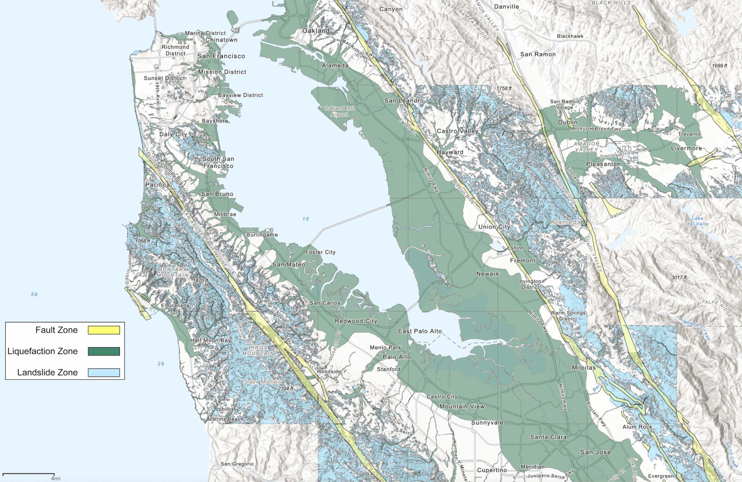
- What areas are prone to liquefaction?
- What areas are prone to landslides?
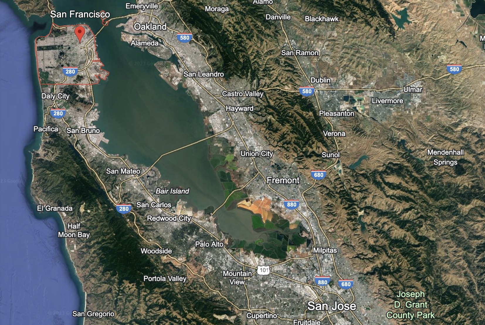
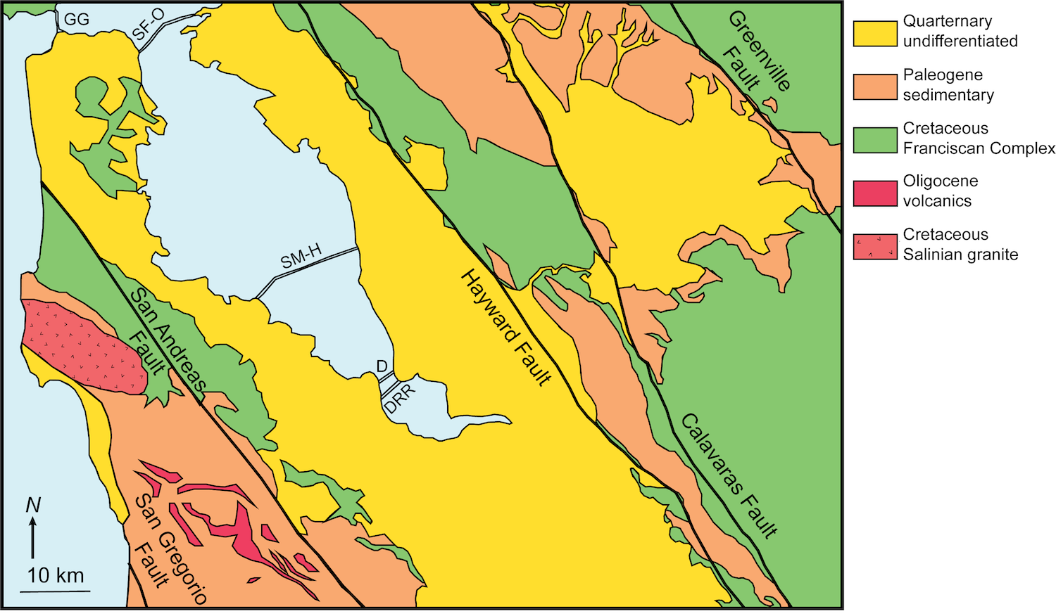
- Compare the Google Earth image (Figure 9.11) and the geologic map (Figure 9.12) to the hazards map (Figure 9.10). Describe some of the relationships between the type of hazard, geologic units, and topography for liquefaction and landslides.
- Choose one of the bridges across San Francisco Bay and determine the geologic hazards associated with both sides of the bridge.
- Your best friend is getting a job in San Ramon CA as a geologist in the headquarters of Chevron. She knows that earthquake hazards abound in CA. The hazard map, however, doesn’t indicate the hazards in this region located on the NE of Figure 9.10. Using the topography and geologic maps (Figures 9.11 and 9.12), let her know what the potential hazards are and where they occur around San Ramon CA.
- Use outside resources to discover some of the historical damage from earthquakes in this region. Which type of hazard was most damaging for these earthquakes? Each group should do one earthquake event and share your results with the class. Some of the events include:
- 1906 M7.9 San Francisco earthquake _________________________
- 1911 M6.0 Calaveras fault Morgan Hill earthquake ________________________
- 1980 M6.0 Livermore earthquake ________________________
- 1984 M6.3 Calaveras fault Morgan Hill earthquake ________________________
- 1989 M7.1 Loma Prieta earthquake__________________________
- 2001 M5.1 Napa earthquake ________________________
- 2007 M5.7 Calaveras fault ________________________
Additional Information
Exercise Contributions
Daniel Hauptvogel, Virginia Sisson, and Kaitlin Thomas
