
Chapter 16: Geophysics
Seismic Waves and Interpretation
Learning Objectives
The goals of this chapter are to:
- Evaluate seismic velocities of common Earth materials
- Understand how to set up and interpret a seismic survey
- Interpret a multibeam bathymetry survey
16.1 Seismic Wave Velocity
Seismology is a branch of geophysics that studies earthquakes and how seismic waves move through the earth. You have already studied earthquakes, so now you need understand how waves move in the Earth. Wave movement is the basis for seismic surveys, which can tell us a great deal about the earth’s subsurface structures. We can learn about the large layers in the earth, such as the mantle and core, or much more locally, like the layers of rock at a building site.
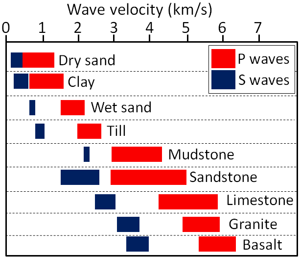
You already know about P- and S-waves from studying earthquakes. The rate these moves (velocity) depends on rock type as well as the temperature, pressure, and orientation of the fabric. Figure 16.1 summarizes the velocity of many common rock types measured at the Earth’s surface.
Exercise 16.1 – Investigate Seismic Velocities
Your instructor is going to demonstrate how to use the V-Meter MK IV. This instrument sends an ultrasonic signal through materials to measure their properties. An ultrasonic signal is a sound that outside our hearing range. In this exercise, you’ll be measuring the P-wave velocities of some common rocks such as gneiss, granite, marble, basalt, gabbro, and sandstone. Chose 3 of these from the samples provided.
- Using a caliper, measure the length of all sides of your samples (x, y, z). Repeat the measurements at least three times and calculate the average distance for each side in mm. Fill in your average length on Table 16.1.
Table 16.1 – Length of materials Material Length x (mm) Length y (mm) Length z (mm) 1: 2: 3: - Determine the density of your sample; density = mass/volume. You can determine the mass by using a scale and the volume by multiplying the three sides you measured in Table 16.1. For this exercise, volume needs to be in cubic centimeters (cm3), so you’ll need to convert your mm3 to cm3 by dividing it by 1000.
Table 16.2 – Density of materials Material Mass (g) Volume (cm3) Density (g/cm3) 1: 2: 3: - Measure the P-Wave velocity through each side of your samples. Record this information on Table 16.3. Calculate the average.
Table 16.3 – P-Wave velocity of materials Material Vx (m/s) Vy (m/s) Vz (m/s) Average (m/s) 1: 2: 3: - Do your velocities match those in Figure 16.1? If not, why might there be a difference?
- Plot your density and P-wave velocity (the x, y, z, and average) data on the graph in Figure 16.2. Use different colors and symbols.
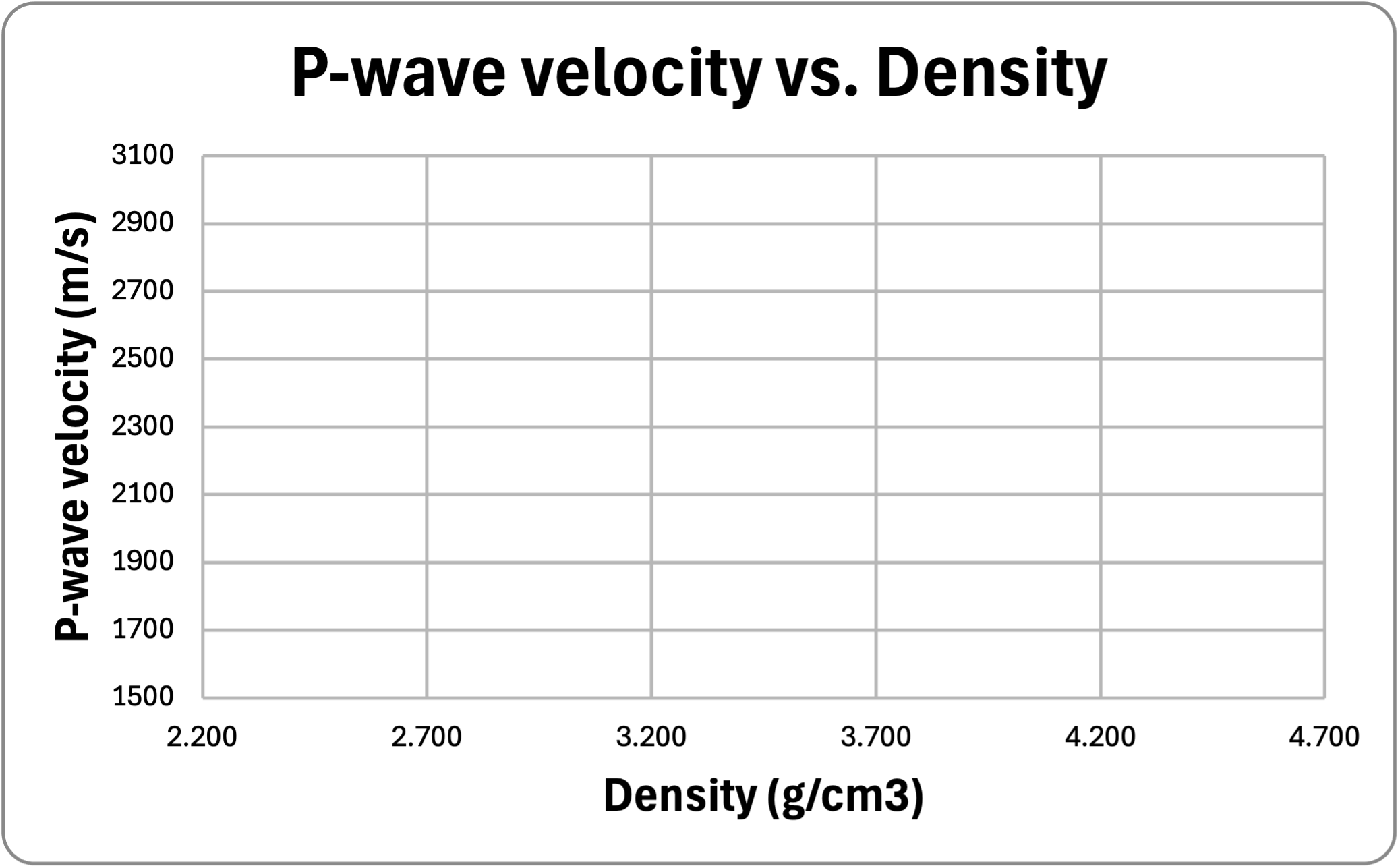
Figure 16.2 – Graph for plotting density and P-wave measurements. - Discuss the relationship between the density of a material and how fast P-Waves move through it.
- Critical Thinking: If you measured P-waves in gneiss, are your P-wave results the same for all directions? Why do P-waves travel faster or slower through different sides of your materials?
- Critical Thinking: Depending on which sample you used, compare P-waves through gabbro versus basalt or granite versus gneiss. Are your results similar or different? Why?
16.2 Seismic Surveys
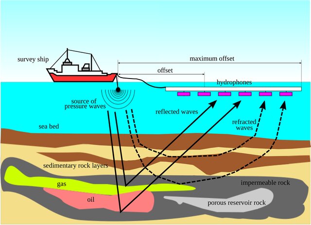
Seismic surveys are used to determine what lies beneath our feet or under the seafloor. They are commonly used in oil and gas exploration, but can also be used to find groundwater sources, investigate locations for potential landfills, determine how an area will shake during an earthquake, and more. These are like CT (computed tomography) scans of the subsurface. Seismic surveys use energy from controlled sources, typically a device that generates vibrations or sound waves. When these energy waves are sent into the Earth, they either reflect or refract through the layers sediment and rock because of differences in density (Figure 16.3). As these waves reflect or refract back to the surface, the energy is recorded by instruments called geophones. The data is then processed and visualized for geologists to interpret (Figure 16.4).
Exercise 16.2 – Conducting a Seismic Survey
Your instructor will set up a seismic survey at the front of the classroom. Use the hammer and record the signal on the seismometer. Notice how the signal changes from the first to the last geophone.
- After the seismometer records the direct wave (called a signal), is this record smooth or noisy? If it is noisy, what is the source of the noise?
- What happens if you change the distance between geophones?
- How can improve the quality (signal to noise ratio) of your shot record?
- Your results only record shallow structure? How would you set up this instrument to determine the deep structure similar to Figure 16.4 or Figure 16.5?
- Critical Thinking: Compare your shot record to those from earthquake seismograms (e.g. Figures 9.4 to 9.6). Why causes these differences?
3-D Seismic Surveys
Seismic surveys can be done in lines or arrays. Arrays are composed of lines at right angles. Why? Well, the result is a 3D image of the Earth (see Figure 16.5). The horizontal layers will show a map view through the area. These may not look like geologic map as these are maps of seismic amplitude. In addition, in the 3D volume, there will cross-sections. In marine 3D seismic surveys, the shooting direction (boat track) is called the inline direction. The perpendicular direction is called the crossline. In marine 3D seismic surveys, commonly, record more than 100,000 traces per square km.
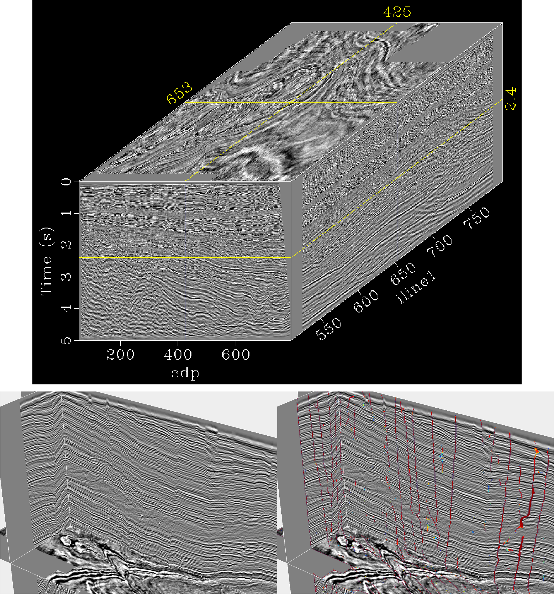
Exercise 16.3 – Interpret a Seismic Survey
The geologic history of the North Sea, between Norway and Great Britain, involves several tectonic events as well as significant sedimentation. In 1976, significant quantities of oil and gas were discovered with center of the North Sea now having many oil and gas wells. Since it is underwater, the only way to figure out what happened is to look at seismic surveys and/or drill holes. As of 2023, there were over 800 wells drilled just in the Norwegian section of this marine basin. Some of these were just for exploration and others have yielded significant quantities of oil and gas.
First look at the stratigraphic column that shows the rock units for this region (Figure 16.6). Each blue, white and red line represents different rock layers with different seismic velocities or amplitudes. using a color scheme with blue for positive amplitudes, red for negative amplitudes, and white for zero amplitude. Notice whether these layers are continuous, discontinuous as well as how bright is the color. These combinations of these features are called seismic attributes or characteristics.
- Describe characteristics of the Neogene units compared to the Paleogene units.
- Describe how you would identify the base of the Cenozoic
- How many distinctive layers are there in the section from Cretaceous to Jurassic? How can you identify the base (bottom) of this sequence?
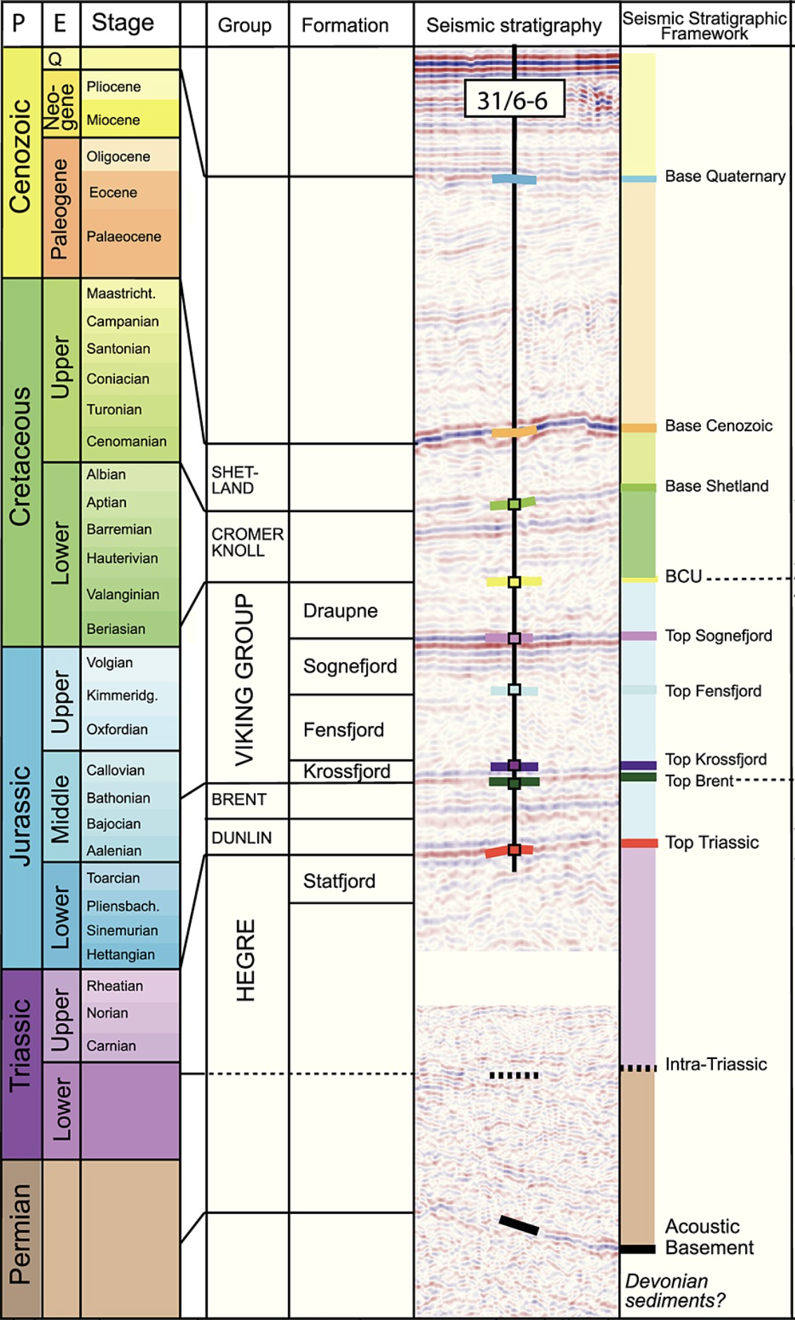
Figure 16.6 – Stratigraphic column with data from well 31/6-6. This well data was used to construct a seismic stratigraphic section for the different rock types. Geologic time is subdivided into P = Period, E = Epoch. In the right-hand column are the boundaries between different units as identified by seismic data. The blue color is used for positive amplitudes, red for negative amplitudes, and white for zero amplitude. Image credit: Bell, Jackson, Whipp and Clements (2014) CC BY. - Now that you can identify the different types of rocks, mark the boundaries between these units on Figure 16.7. If the layers are not continuous, there may be faults or folds.
- Identify and mark at least 3 faults on this figure. What type of faults? What is the tectonic environment?
- Are there any unconformities in this seismic section? If so, what type?
- Critical Thinking: Why are there so many drill holes in this area?
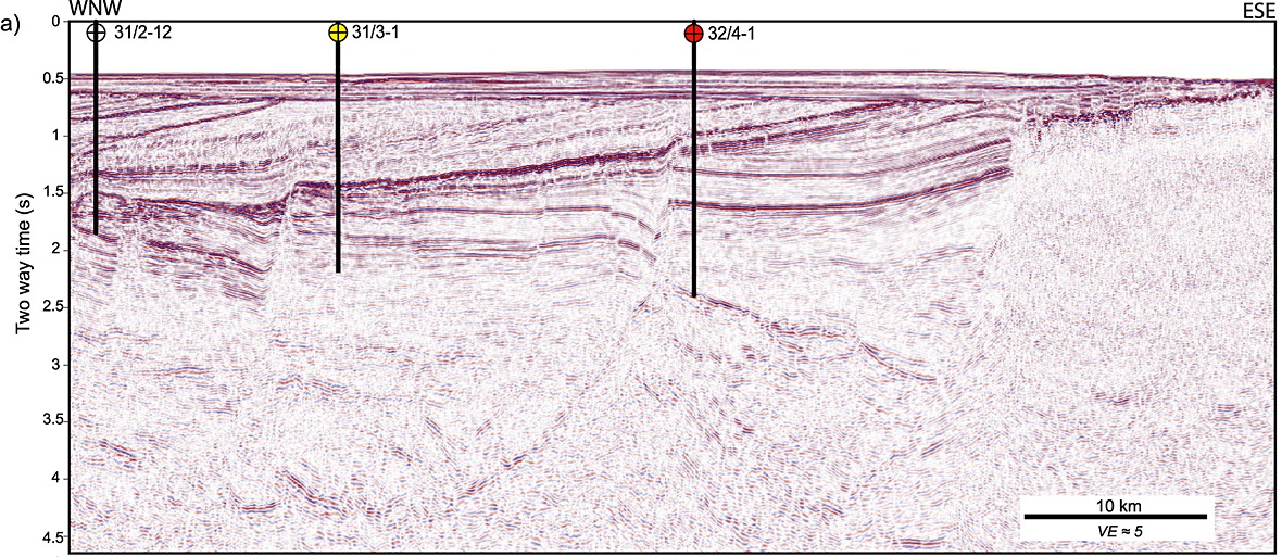
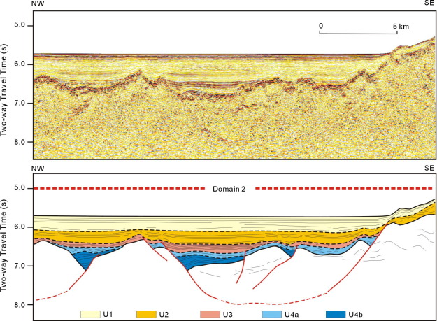
Figure 16.7 Uninterpreted 2D seismic reflection profile across the Horda Platform in the North Sea between Norway and Great Britain. The vertical axis represents the time it took for the seismic energy to be recorded at the geophone array. The white area at the top is the ocean. The colored lines represent different seismic amplitudes with blue for positive amplitudes, red for negative amplitudes, and white for zero amplitude. The vertical lines are locations of drill holes. VE = vertical exaggeration. Since this is vertically exaggerated, dipping lines will appear steeper than they actually are. Image credit: Bell, Jackson, Whipp, and Clements (2014)
16.3 Sonar
So far, you’ve only had exercises about seismic waves but there are many other physical properties that can be used to study Earth such as gravity, magnetics, and electricity. These all can be used to study what is below the Earth’s surface. Instead, let’s do one final exercise to study the surface of the Earth. You’ve seen many topography maps in this lab manual. Ever wonder how these are made? Now, most surface elevation data is obtained using data from satellites, or satellite altimetry. These use either radar or sonar signals to measure heights (altimetry). Another technique is to use sonar instruments that are towed behind ships to map the seas floor. For the oceans, much of this data is in a national repository, Global Multi-Resolution Topography (GMRT). As of May 2024, this web site had data for 40,838,234 square kilometers of multibeam sonar data from 1,490 cruises! This may seem like a lot of data, but it is only about 8% of the area of all oceans. So, there is a lot we don’t know about the ocean floor.
Exercise 16.4 – Interpret Multibeam Sonar Surveys
Ocean basins have lava flows erupted a mid-ocean ridges and volcanos scattered throughout them. There are so many volcanos that most are unnamed. The world’s tallest volcano is Mauna Kea measured from the ocean floor to its peak on the Big Island of Hawaii. These volcanos can be used to learn about the history of ocean basins as well as magmatism in these areas.
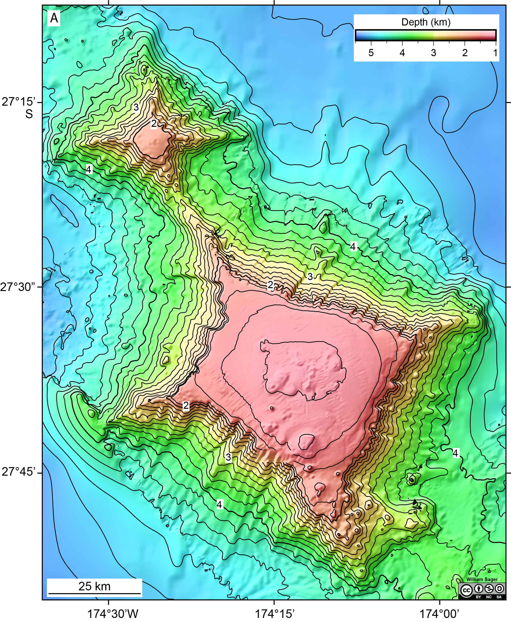
First look at Figure 16.8.
- Describe the characteristics of this volcano including its height above the sea floor and its approximate volume using the formula for a cone (⅓ 𝜋r2h) with r for radius and h for height.
- Using this information can you determine if this is an old or young volcano?
- Go look back and look at Figure 6.8 and your results from Exercise 6.5. Do you think this volcano is the result of one or many eruptions? How did you determine this?
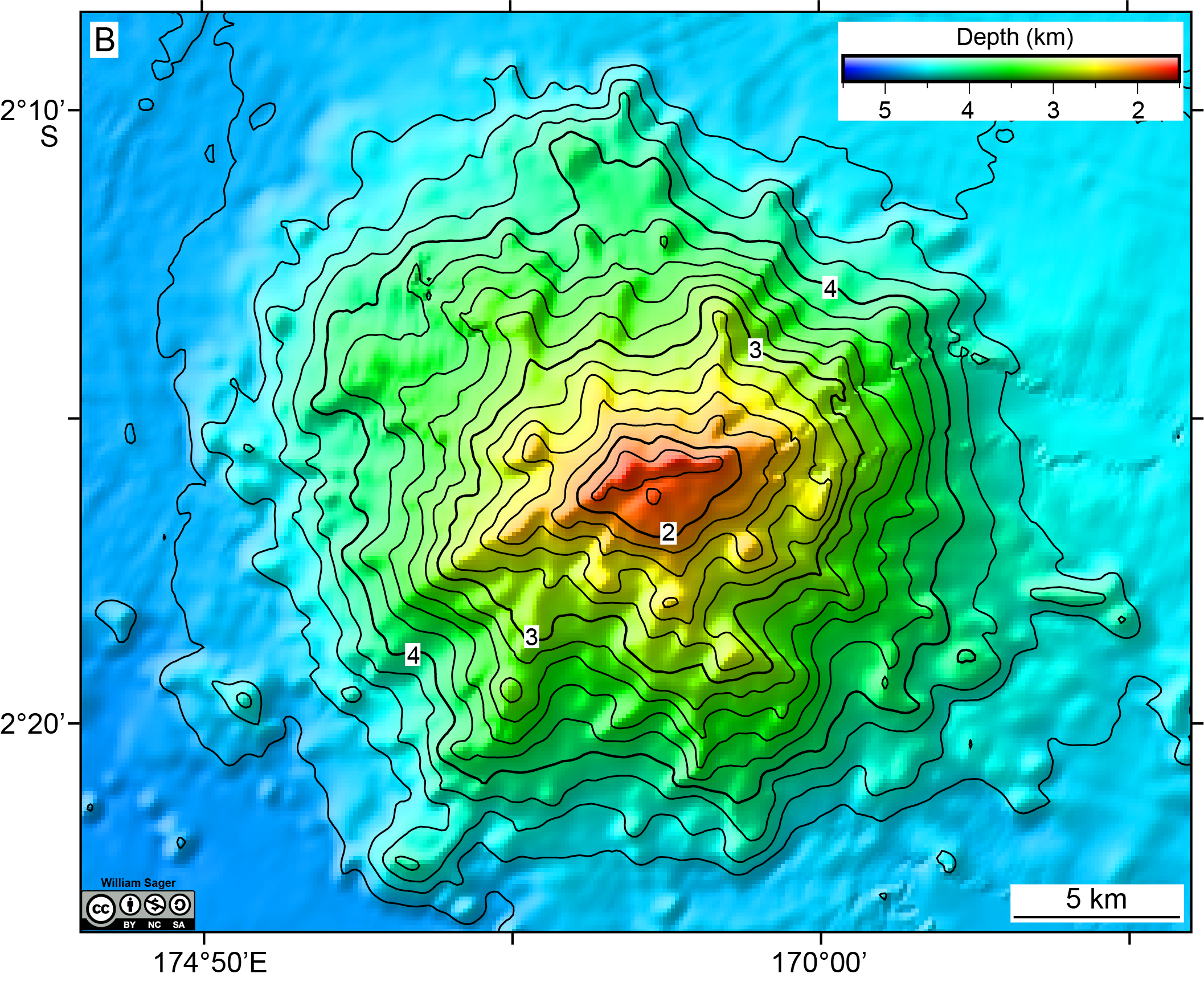
Figure 16.8 – Schematic color-coded bathymetric map of an unnamed volcano in the Pacific Ocean. Note that the colors correspond to depth beneath the ocean surface with cooler colors for deeper depths and warmer colors for shallower depths. Contour intervals are 200 m, with thicker lines at 1 km intervals. Image credit: William Sager, CC BY NC SA.
The Louisville Ridge is an underwater chain of over 75 seamounts located in the southwest Pacific Ocean. It stretches for 4,300 km (2,700 mi) making it the longest seamount chain on Earth. Remember exercise 3.6 about the Hawaiian hotspot. Well, this volcanic chain results from movement of the Pacific Plate over the Louisville hotspot. The volcanos range from 77 Ma at the NW end of the chain to 1.1 Ma at its SE end; this is age spread is similar to the Hawaiian Emperor seamount chain. In lecture, you may have learned about how some oceanic volcanic islands erode and form guyots (flat topped volcanoes) and then coral atolls. So, the shape of the volcano may help you determine its age. To do this you need to determine if the volcano was ever high enough to be above the sea floor. Examine the two volcanoes in Figure 16.9.
- Describe the characteristics of these two volcanoes including their height above the sea floor and their approximate volume using the formula for a truncated cone (⅓ 𝜋[(r2+r) x (R2+R)]h) with h for height, r for radius of the top of the flattened area and R is the radius for the bottom of the volcano.
- These two volcanoes have features that look like spokes of a bicycle wheel. How did these form?
- Do you think these flat-topped volcanoes (guyots) were formed by eruption or by erosion. Why?
- Critical Thinking: How much magma was erupted in the two areas? Compare the volcanoes in the Figures 16.8 with 16.9, especially their volume. Do you think the oceanic lithosphere has different thickness in the two areas?
Additional Information
Exercise Contributions
Virginia Sisson, Daniel Hauptvogel, Yin-Kai Wang, Andrea Paris
References
Bell, R.E., Jackson, C. A.-L., Whipp, P.S., and Clements, B., 2014, Strain migration during multiphase extension: Observations from the northern North Sea, Tectonics, v. 33, p. 1936-1963 DOI: 10.1002/2014TC003551 CC BY.
