
4.4 Preparing to Print
Learning Objectives
- Review each worksheet in a workbook in Print Preview.
- Modify worksheets as needed to professionally print data and charts.
In this section we will take a look at each of the worksheets created in the previous sections. Since these worksheets contain a combination of data and charts, there are specific things to watch for if you will be printing the sheets.
We will start by looking at each worksheet in Print Preview in Backstage View. We will then make any changes necessary, such as changing the orientation and scaling, or moving charts around on the worksheet. To make sure we don’t miss any worksheets, we are going to review the worksheets in the order they appear in the tabs.
Previewing Chart Sheets for Printing
Data file: Continue with CH4 Charting.
The first worksheet, Closing Prices, is a chart sheet. This means that it does not contain any data; remember that chart sheets just contain charts. We still need to review it in Print Preview.
- Click on the Closing Prices worksheet tab.
- Go to Print Preview by clicking Print in Backstage View.
- Notice that the chart will print on the entire page, in Landscape orientation.
- There is nothing to change. Exit Backstage View.
Printing Worksheets with Data and Charts
The next worksheet (Stock Trend) has a lot of data and multiple charts. We need to print the data and the charts, which will require some modifications of the page setup.
- Click on the Stock Trend worksheet tab.
- Go to Print Preview by clicking Print in Backstage View.
- Notice that this worksheet is currently printing on seven pages.
- As you click through each page you should make the following observations:
- The data is split between the first and third pages.
- The line chart starts on the first page, but part of it is also on the second page.
- The double-line chart starts on the third page, and then finishes on the fifth page.
- The fourth and sixth pages are blank.
- The last page has a column of seemingly random numbers.
- Exit Backstage View.
The first thing we are going to do is remove the numbers that are appearing on page 7. To do this, we will hide the column where they are being stored. We are going to hide the column, instead of deleting the numbers, in case the numbers are being utilized somewhere else in the workbook.
- Scroll to the right on the worksheet until you find the numbers in column AH.
- Click anywhere in column AH.
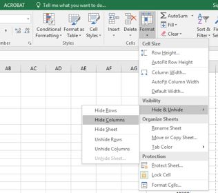
- On the Home ribbon, click the Format button in the Cells group.
- In the Visibility section, select Hide & Unhide then select Hide Columns (see Figure 4.64).
- The visible column headings should now go from AG to AI.
- Return to Print Preview in Backstage View to see the changes to the printed worksheet.
- Notice that there are now five pages. The data and charts are still splitting across multiple pages, but the numbers in column AH are no longer going to print.
- Remain in Backstage View for the next steps.
The data is still split between pages 2 and 3, and the charts are splitting oddly as well. The first step we will try to fix these issues is to change the page orientation and scaling.
- While still in Backstage View, change the page orientation to Landscape (use the Orientation drop-down menu in the Settings section).
- This puts all of the data on one sheet, but the charts are still split between multiple pages.
- Change the page scaling to Fit Sheet on One Page (use the Scaling drop-down menu in the Settings section).
- This fits everything on one page, but it is too small to be able to read.
- Change the page scaling back to No Scaling.
The next thing we will try is moving one, or both, of the charts. In order to move the charts, we need to exit out of Backstage View.
- Exit Backstage View.
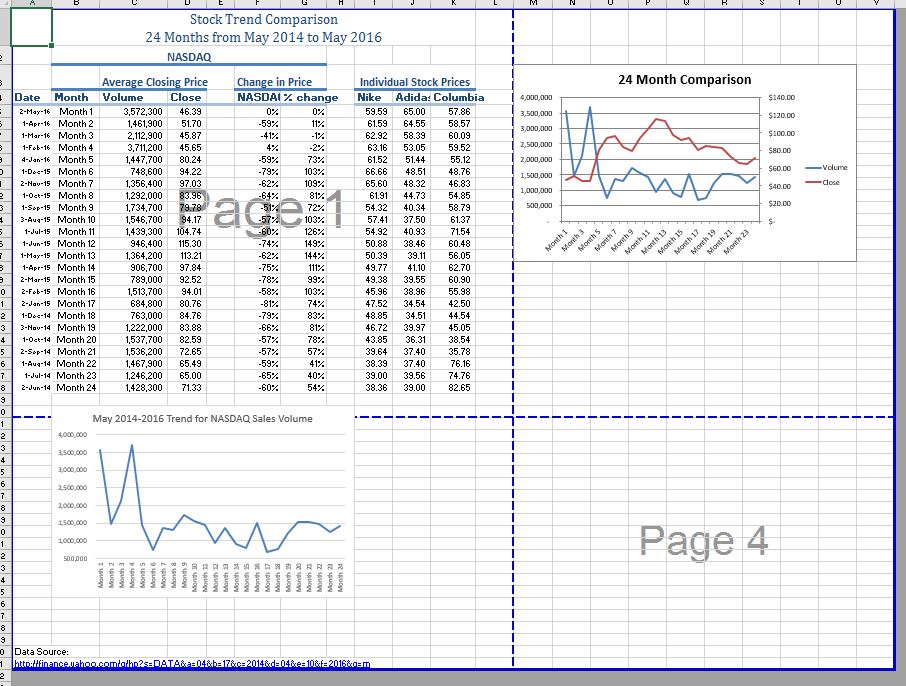
- Switch to the View ribbon and then select Page Break Preview. Your screen should look similar to Figure 4.65. (Remember that the dotted blue lines indicate automatic page breaks.)
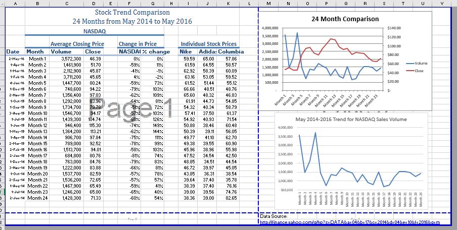
- Move the 24 Month Comparison (double-line) chart closer to the top of its page.
- Move the May 2014-2015 Trend for NASDAQ Sales Volume (line chart) so that it is under the 24 Month Comparison chart.
- The link to the data source is still at the bottom of page 2 (in A50:A51) so you need to move it as well. Using your preferred method, move the text from A50:A51 to M31:M32.
- Now your screen should look similar to Figure 4.66.
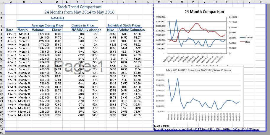
We don’t want the data source link text to print on its own page, but there is no room to move it onto the same page as the charts. To fix this, we are going to remove the automatic page break between the charts and the text in M31:M32.
- Place your pointer on the horizontal blue dashed line (automatic page break) between the line chart and the Data Source link text.
- When your pointer changes to the double arrow (pointing up and down), drag the page break down into the gray area. This removes the page break.
- If your vertical automatic page break between columns L and M moves, drag it back between columns L and M. This will make it a solid blue line, which will no longer adjust automatically.
- Your screen should now look like Figure 4.67.
Now you need to do one final check of this worksheet in Print Preview.
- Go to Print Preview and look at both pages. Page 1 should contain just the data and page 2 should have both charts and the Data Source link text.
- Exit Backstage View and save the file.
Preview Remaining Worksheets for Printing
There are four remaining worksheets to be reviewed. Some of them will need minor changes and some will not need any changes. You will need to preview each one and then make the specified changes. In the following steps you will preview and modify the next three worksheets.
- All Excel Classes – this is a chart sheet, so it should not need any changes.
- Grade Distribution – the chart is split across two pages. Fix this by changing the orientation (Landscape) and scaling (Fit Sheet on One Page).
- Enrollment by Race Chart – this is a chart sheet, so it should not need any changes.
Printing a Chart Only
Sometimes you might have a worksheet that has data and a chart, but you only want the chart to print. That is the case with the Enrollment Statistics worksheet.
- Switch to the Enrollment Statistics worksheet.
- Select the chart.
- Go to Print Preview. Only the chart is printing. (If it shows the data printing along with the chart, exit Backstage View and be sure to select just the chart on the worksheet.)
- If needed, change the orientation to Landscape. This orientation looks better when printing just a chart.
- Exit Backstage View.
Hiding a Worksheet
You have actually decided that you do not want the Enrollment by Race Chart sheet to be visible at all, but you do not want to delete it. We are going to hide it from anyone looking at the workbook.
- Right-click on the Enrollment by Race Chart tab.
- Select Hide from the menu that appears. The Enrollment by Race Chart sheet should no longer be visible.
- Now you want to bring the worksheet back. To unhide it, right-click on any other worksheet tab and select Unhide from the menu. A list of hidden worksheets will be displayed. Select the Enrollment by Race Chart and click OK.
- Save the CH4 Charting workbook.
- Compare your work (on all of the worksheets) with the self-check answer key (found in the Course Files link).
- Submit all three files from this chapter (CH4 Charting.xlsx, CH4 Diversity in Enrollment in Community Colleges.docx, and CH4 Diversity in Enrollment in Community Colleges.pptx) as directed by your instructor.
Attribution
“4.4 Preparing to Print” by Julie Romey, Portland Community College is licensed under CC BY 4.0
Media Attributions
- figure-4-64
- figure-4-65
- figure-4-66
- figure-4-67
