1 Chapter 1: Introduction
Jiajia Sun; Xinyan Li; and Felicia Nurindrawati
1.1 Learning objectives
Hello, everyone. Welcome to the potential field class! In this class, we will focus on the fundamental theory and commonly used data processing and interpretation techniques in potential field methods. This class consists of both lectures and lab exercises. After completion of the class, students can expect to
- Understand the fundamental theory behind potential field methods;
- Understand gravity and magnetic data acquisition practices, instrumentation and processing procedures;
- Understand various data processing techniques in Fourier domain;
- Be familiar with various interpretation methods for depth estimates;
- Be able to use Geosoft software to perform 2D basin modeling;
- Understand the 3D inversion theory and methods for potential field data; and
- Be familiar with various applications of potential field methods.
The target audience of this course is anyone who is interested in learning more about
- fundamental potential field theory;
- Processing and interpretation methods; and
- Application examples of potential field methods to
- Petroleum;
- Mineral;
- Geothermal;
- Geotechnical/Engineering (e.g., caves and tunnels);
- Regional to continental-scale geological studies; and
- Environmental (e.g., unexploded ordnance UXO)
1.2 Potential
Both gravity and magnetic fields can be described using a quantity called potential. Potential is a scalar and obeys Laplace’s equation in source-free regions. Therefore, these two methods are collectively referred to as potential field methods in the geophysics community.
The fact that potentials are scalar quantities makes it easier to deal with the mathematics involved. After all, working with scalars is always easier than working with vectors. Note that, both gravity and magnetic fields are vector fields because gravity not only has a magnitude (such as 9.8 m/s2) but also has a direction; the same is true for the magnetic field.
1.2.1 Geophysical signals
Geophysical signals are mostly produced by contrasts in some physical properties of Earth materials. For example:
- Variations in electrical conductivities of the subsurface rocks produce secondary potentials that can be measured in a DC survey and used for subsurface imaging;
- Differences in the reflectivity/absorption of near-surface Earth materials result in useful remote sensing images;
- Changes in acoustic impedance between Earth materials result in seismic reflections.
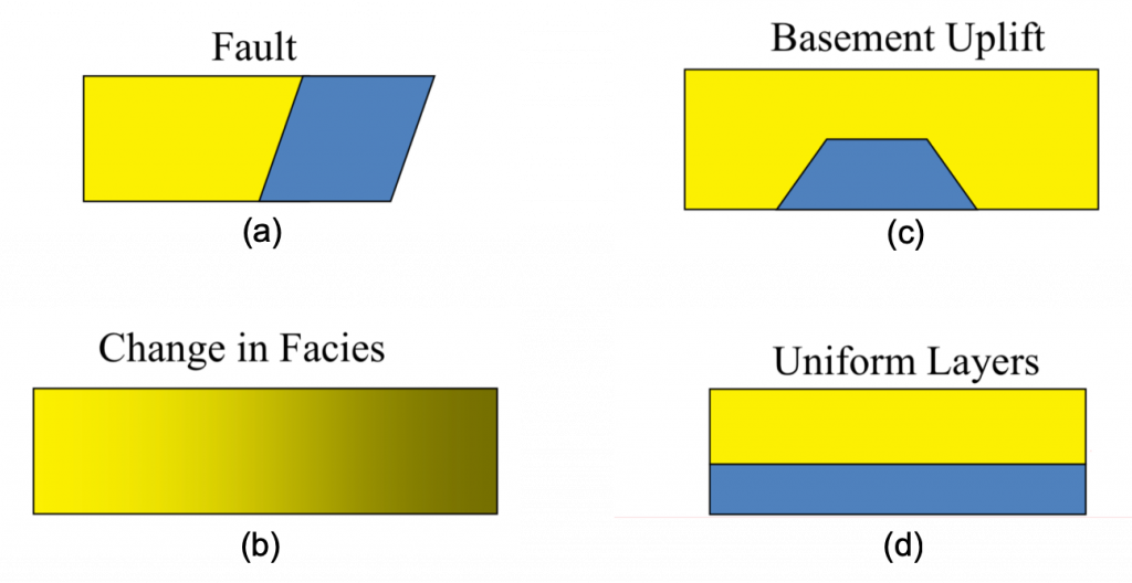
Specifically, in gravity & magnetic methods, the material properties to be considered are density and magnetization (magnetic susceptibility), respectively. Signals result from horizontal changes in the density and magnetization of the Earth materials can be used for detecting lateral changes produced by either vertical displacement of homogeneous layers or by inherent lateral inhomogeneities in the Earth materials themselves, as model examples shown in figure (a, b, c) below. However, horizontal layers with constant properties (figure (d)) provide no signal and consequently are “invisible” to the gravity and magnetic methods.
In fact, we should be aware that, the above statements are only true for surface gravity and magnetic measurement. If there are borehole gravity and magnetic measurements, potential field methods can be used for detecting physical property changes in the vertical direction. More details on borehole gravity can be found in https://wiki.aapg.org/Borehole_gravity, and some borehole gravity applications can be found here.
1.3 Application examples
There are many applications of potential field methods. In the following, we will discuss some major geoscience applications.
1.3.1 Application to oil, gas and groundwater studies
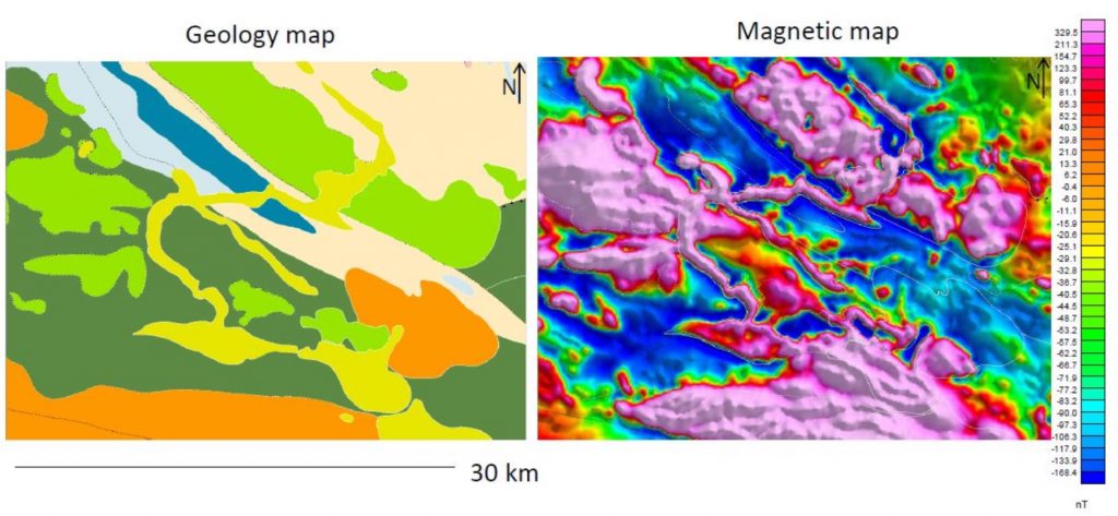
Example 1: Geologic mapping
Geologic contacts can be quickly inferred from the magnetic maps, as illustrated in the figure below (image credit from Douglas Oldenburg at UBC).
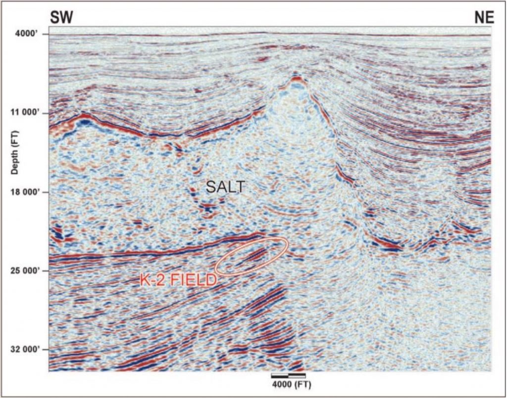
Example 2: Salt dome imaging
In many Gulf of Mexico prospects, salt plays a key role in acting as a structural trap. Overhanging salt often forms seals, and sediments on salt flanks can have structural and stratigraphic pinch-outs against the salt. The exact shape of the salt is critical in understanding these traps. Unfortunately, seismic imaging often tends to be poor in these prospects. The seismic image from O’Brien et al., 2005, TLE, illustrates the limitation of interpreting the salt dome using seismic imaging alone.
Example 3: Groundwater studies
Time-lapse gravity data, also known as 4D gravity data (with the 4th dimension being time) is often used to monitor the movement of water underground. Time-lapse data can be obtained by conducting multiple surveys in the same location but at different times. Besides gravity data, there are other methods that can be used to monitor groundwater movement. However, due to the delay in signal responses of the groundwater movement, some methods might be less effective than others. According to a study conducted by Kenedy, 2016, time-lapse gravity is “the most sensitive to movement of water through an unsaturated zone”.
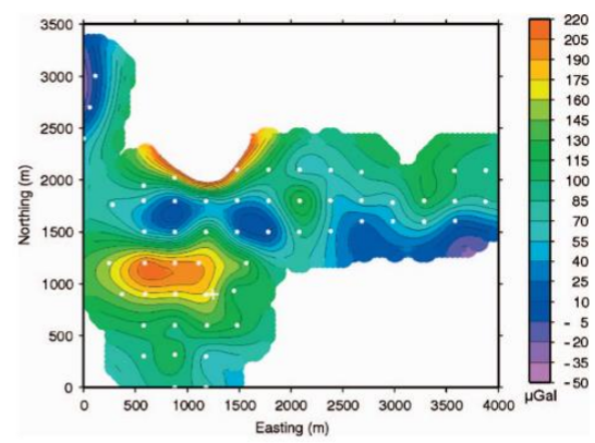
One example of groundwater monitoring with time-lapse gravity approach is shown in Davis & Li, 2008. In this paper, the movement of water injected into an underground artificial aquifer storage system is monitored using time-lapse microgravity data (meaning that the data obtained is in the orders of micro-Gal). The following figure shows the total gravity difference between April 2004 and February 2005, and the white (+) indicates the location of the injection well. We see that there is a positive gravity difference around the injection well, spanning towards the north-west side, which is the direction of the water injected into the reservoir.
Example 4: Reservoir waterflood surveillance
One of the most notable use of the 4D microgravity method is the time-lapse microgravity survey at Prudhoe Bay, Alaska (Hare, 2008) In this case, the gas production in the field started to decline. It was suspected that there might be something wrong with the water injection which is used to maintain pressure, and therefore maintain production. The problem is that there were only a few wells available in the area that can be used to monitor the water movement in the reservoir. With that, they considered the use of gravity survey to monitor the waterflood movement in the reservoir. The figure below shows density models obtained through inversion (with each figure showing different inversion results using different inversion constraints). The method was successful in determining the behavior of the waterflood movement in the reservoir. 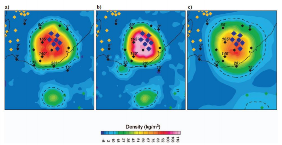
1.3.2 Application to mineral exploration
Gravity and magnetic survey are especially useful in mineral explorations, as they have useful features that are not offered by seismic surveys, such as how gravity and magnetic surveys can cover a massive geographical region in just a couple of days with surveys conducted using airplanes. Examples for the use of gravity and magnetic surveys in mineral exploration are:
- Sulfide exploration
Massive sulfide deposits that came from volcanic sources and are rich in copper, zinc, lead and can contain other precious metals such as gold and silver (mining.com). The deposit is very high in density in comparison to the background, and thus a gravity survey is generally done for these types of target. The following figure is the gravity data obtained from a massive sulfide as well as the cross-section of the interpreted geology (credit: Yaoguo Li)
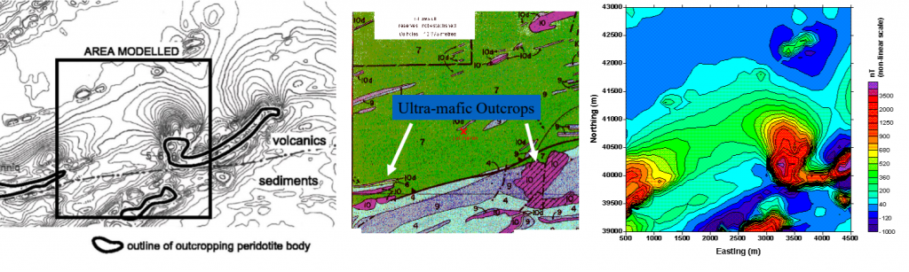
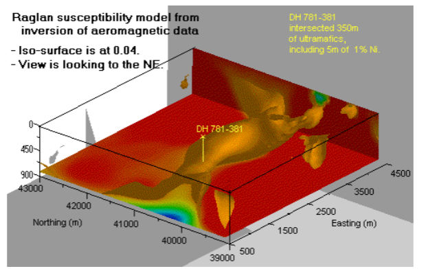
Due to the magnetic properties of the massive sulfide, magnetic surveys can also be done for this type of target. The following figure shows the aeromagnetic data of the Raglan deposit, a well-known nickel copper deposit in Canada (Watts, 1997). One of the questions posed for this region is whether the peridotite outcrops (appear in purple on the surface geologic map) are connected at depth or not. This is an important information to know the optimum location for drilling.
After inversion of the magnetic data, it is found that the outcrops are connected at depth and the drill hole can then be placed according to the interpretation from the inversion results.
- Iron exploration
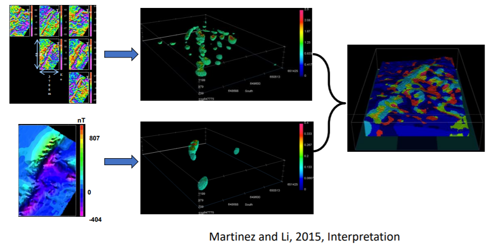
Other examples of gravity and magnetic data used in mineral exploration would be Iron exploration (Martinez and Li, 2015). The following Figure is the gravity gradient tensor data and the magnetic data for a geographical region as well as the inversion results.
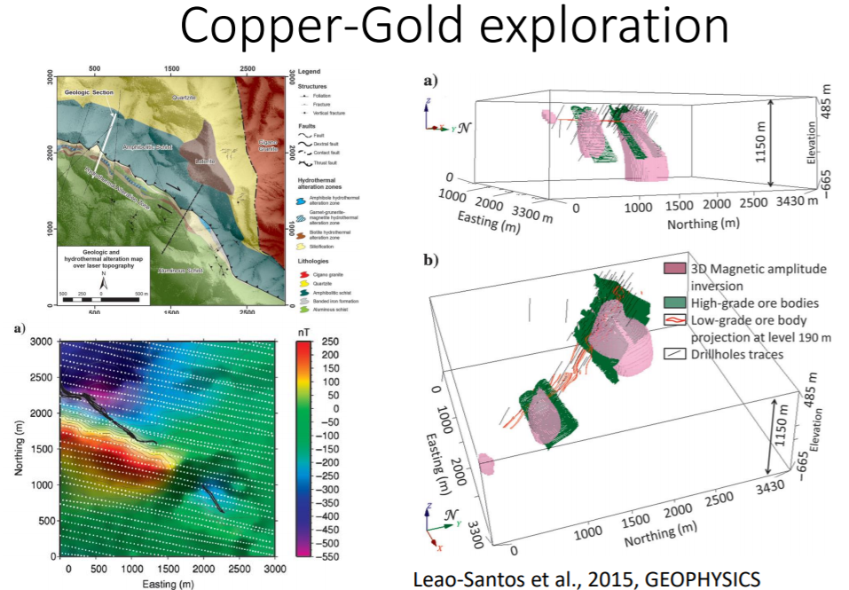
- Copper-Gold exploration
Another example is from Copper-Gold exploration (Leao-Santos, 2015). The following figure shows the geologic map as well as the magnetic data of the region. We see that the overall trend in the geologic map is also apparent in the magnetic data map. Figure (a) and (b) showcases the 3D inversion results of the magnetic data and the interpretation based on the inversion result.
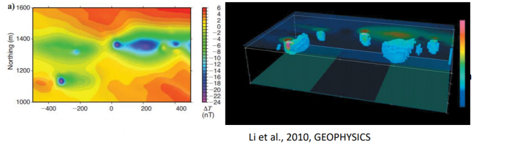
- Diamond Exploration
Diamonds are typically found in kimberlite pipes, which are igneous rocks with magnetic properties. From the following figure, we can see that the Total Magnetic Intensity (TMI) data has outlined an elongated body indicated with the negative anomaly values in Figure (a). After inverting the magnetic data, we can see the two broad elongated sources, interpreted as the kimberlite dikes. The vertically oriented bodies represents the kimberlite pipes in the region.
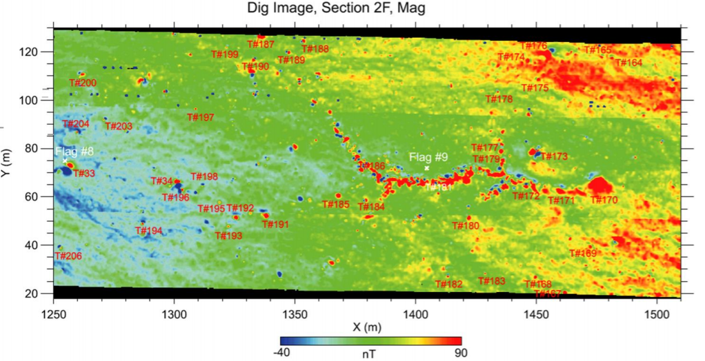
- UXO Detection
UXO (Unexploded ordnance) are explosive weapons, such as bombs, missiles, grenades, that did not explode during deployment, but poses high risk of detonation even decades after it was buried underground. Fortunately, UXOs are highly magnetic and thus we can detect them by conducting magnetic surveys over the region of interest. The following are examples of UXO data (credit: Yaoguo Li)
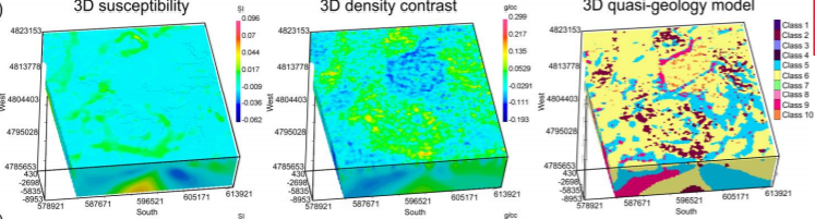
1.3.3 Basement characterization
Basement characterizations are done by interpreting the basement geology of a certain region based on the data obtained in the survey. Gravity and magnetic surveys can cover extensive geographical regions in a matter of days (using airplane or helicopter). Using inversion, the distribution of density and the magnetic susceptibility of the region can be found. Potential resources can be interpreted based on the recovered physical parameters, as certain geological units have a known range of density and magnetic susceptibility values. The following figure shows a 3D magnetic susceptibility model and 3D density contrast from inversion results and the interpreted geological units based on the the inversion results.
1.3.4 Cave Detection Example
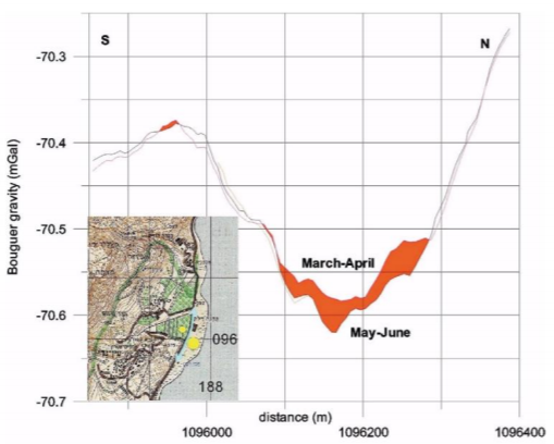
Sinkholes are a serious environmental problem and hazard, especially around the Dead Sea area. The largest sinkhole found in the region was as large as 30m in diameter and 15 m deep. The recent collapse on both sides of the main highway at E’n Gedi, a popular destination for recreation and tourism, poses a risk for many people in the region. The sinkholes initially opened at a campsite east of the road, and subsequently, several sinkholes opened west of the road, which indicates that there might be a possible collapse of the highway in the near future. Gravity method is especially useful for this case. Having a hole underground surely will create a large density contrast (essentially replacing the rocks underground with air, a substance with a very low density). The following figure shows a time-lapse gravity data. The gap between the gravity data between March-April and May-June indicates the development of sinkholes happening in the region of study (Rybakov et al., 2001).
1.4 Advantages of potential field methods
In comparison with other geophysical methods, such as seismic exploration, there are a lot of advantages of potential field methods that make it attracting, for example:
- it is inexpensive;
- measurements can be covered a large area in a short timeframe;
- signal sources are passive and non-destructive, we do not need to create any man-made sources;
- quick interpretation can be made;
- global coverage data, etc.