
5 Chapter 5: Fourier-domain Modeling & Transformations
5.1. background
5.1.1. Motivation
Up until this point, we have dealt with 2D gravity and magnetic data maps in the spatial domain. In this chapter, we will be looking at different way in dealing with these data: in the frequency domain. A lot of data processing techniques require the data to be in frequency domain due to its simpler and more efficient mathematical operators. The motivation to studying Fourier domain modeling for modeling any potential fields data are the following:
- The expression of potential field in frequency domain gives us a different perspective to look at our data
- Much of the processing and analysis of potential field data are done in frequency domain
- Potential field is related to the source distribution by a convolution with the Green’s function (will be explained later on)
In this chapter, we will examine Fourier expression of simple potential functions and Fourier expression of field due to simple sources.
5.1.2. frequency and phase
Before going over Fourier Transforms, we first need to know the basic theory behind it. There are several basic concepts that we will first cover before going through Fourier transforms.
5.1.2.1. Waveforms
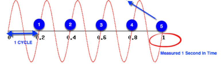
A spring-mass system, as we see in the figure below, oscillates throughout time. The displacement of the mass from the oscillatory behavior can be graphed with respect to time as we see in the figure. It turns out this movement can be expressed as a sinusoidal function. We call this a waveform.
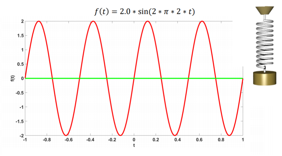
The amplitude of the waveform depends on the constant before the sin function. For example, the above figure shows an waveform with an amplitude of 2 units. The blue value in the below indicates the amplitude.
f(t)= 2.0 *sin (2* π*2*t)
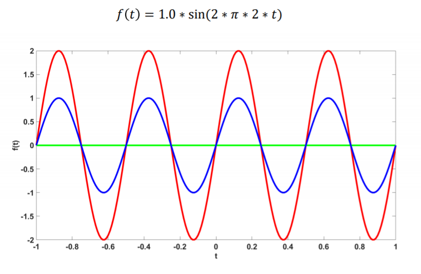
If there is a function that has the form of f(t) = 1.0*sin(2*π*2*t), then the waveform will be exactly the same as the aforementioned example, except that the amplitude would be halved, as we can see in the blue line in the following figure:
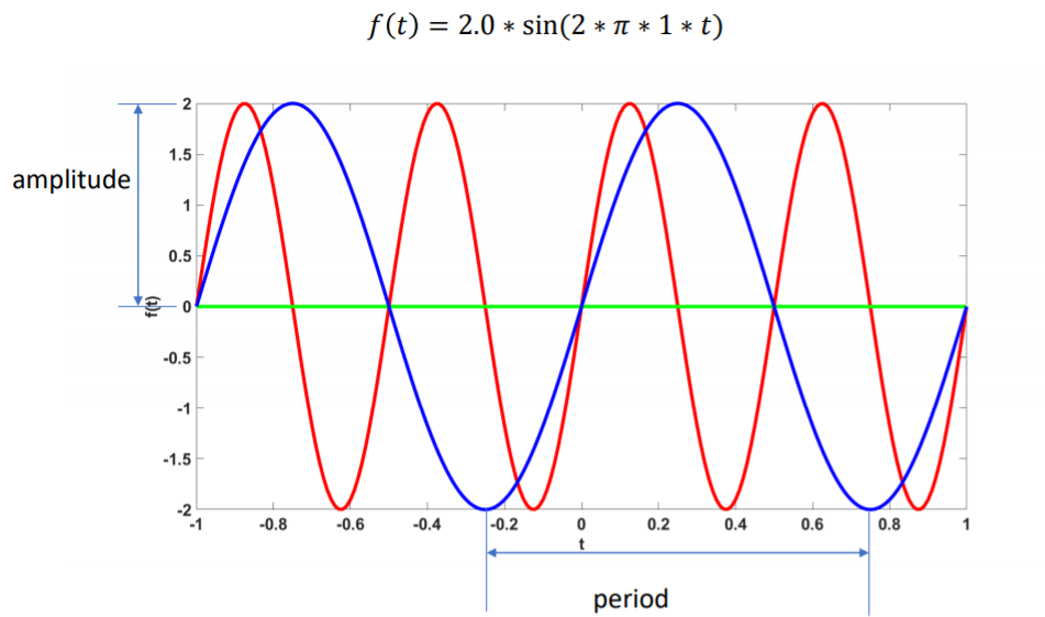
The period of the waveform depends on the value preceding t inside the sin function . One period represents the amount of time it takes for the waveform to undergo one cycle (1 peak and 1 trough). For example, the red text in the following waveform determines the period:
f(t) = 2.0 * sin(2* π *2*t)
If there is a function that has the form of f(t) = 2.0*sin(2*π*1*t), then the waveform will be exactly the same as the aforementioned example, except that the period is twice of that, as we can see in the blue line in the following figure:
5.1.2.2. Frequency
The frequency of the waveform can be determined by the period. Frequency represents the number of cycles in one second, and the unit is (/s) or Hertz(Hz). Frequency can also be mathematically defined as:
f = 1/T
Where T is the period.
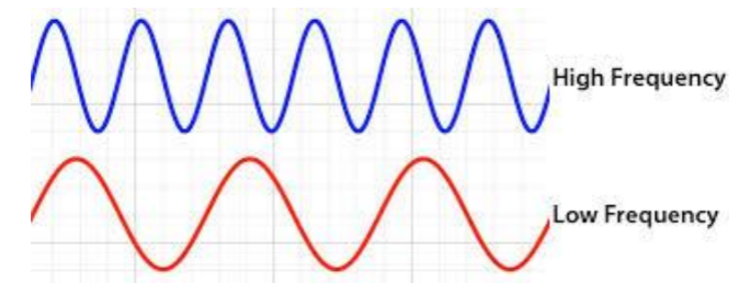
If we have waveforms that have their peaks and troughs closer together, we say that the waveform has a high frequency. If they are far apart, then the waveform has low frequency.
Test your understanding: frequency
 What is the frequency of this waveform? What about the period?
5.1.2.3. Phase
Phase is determined by the argument inside the sin function. For example, the following figure shows two waveforms of different phases. The first function below is for the red line in the graph, and the second one is for the blue line in the graph.
f(t) = 2.0 * sin(2 * π * 2 * t)
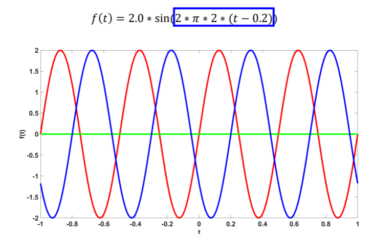
Notice that the two waveforms have the same amplitude and frequency, but one seems to be delayed compared to the other. This is because these two waveforms have different phases.
Phase is the argument inside the sine(or cosine) function for a waveform. Given a fixed amplitude and frequency, phase determines when the peaks (or troughs) occur. Simply, it specifies where in the cycle is it oscillating at t=0. The unit for phase is in degrees or radians.
There are two terms that are related to phase: in-phase and out-of-phase.
If the two peaks of two signals with the same frequency are in the exact same alignment at the same time, then they are called in-phase. If the two peaks of two signals with the same frequency are not in an exact alignment at the same time, then they are out-of-phase. The following figure gives out a visualization of the two difference.
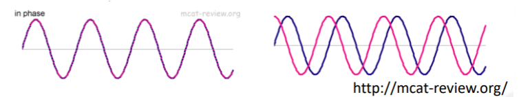
The important concept that we want to take home from this is the fact that a sine wave and a cosine wave are 90 degrees out-of-phase with each other. Thus, we can express a waveform in two ways: using a sine wave or a cosine wave.
5.1.2.4 General notation
The more general notation of a waveform can be expressed as:
![\[f(t) = A sin(\omega t + \phi)\]](https://uhlibraries.pressbooks.pub/app/uploads/quicklatex/quicklatex.com-e37f2b84ea1e50af58a5e4e7fe93161b_l3.png "Rendered by QuickLaTeX.com")
![\[f(t) = A cos(\omega t + \phi)\]](https://uhlibraries.pressbooks.pub/app/uploads/quicklatex/quicklatex.com-5780798573ab9a3d1dfae342c1912b7d_l3.png "Rendered by QuickLaTeX.com")
Where A is the amplitude, and  is the angual frequency in radians per seconds. The angular frequency can be found from the equation:
![\[\omega = \frac{2\pi}{T} = 2\pi f\]](https://uhlibraries.pressbooks.pub/app/uploads/quicklatex/quicklatex.com-4314680e066c9854c0d07d5210cca49c_l3.png "Rendered by QuickLaTeX.com")
Main takeaways from this frequency and phase
Any periodically oscillating sinusoidal wave can be characterized by three fundamental properties
- Amplitude(A)
- Frequency(
 )
) - Phase(
 )
)
A wave can be expressed using the following notation:
f(t) = A sin(ωt + φ)
or
f(t) = A cos(ωt + φ)
5.1.3. complex variable
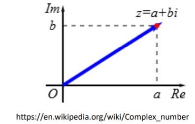
A complex variable can be expressed as such:
![\[z= a+ib\]](https://uhlibraries.pressbooks.pub/app/uploads/quicklatex/quicklatex.com-2475ea83d1bc71f900f1ae087f5a0a2b_l3.png "Rendered by QuickLaTeX.com")
where a and b are real numbers, and i is the imaginary unit that is equal to  , thus
Thus, a complex number can be separated into two:
- a: real part
- b: imaginary part
A complex number can be viewed as a point in the complex plane, as the following figure:
5.1.3.1 Absolute value and argument
We know that a complex number can be expressed as such:
![\[z = a + ib\]](https://uhlibraries.pressbooks.pub/app/uploads/quicklatex/quicklatex.com-30420f525d00abd8c343195f7db119c6_l3.png "Rendered by QuickLaTeX.com")
The absolute value(modulus) of this complex number is thus:
![\[|z| = r = \sqrt(a^2 + b^2)\]](https://uhlibraries.pressbooks.pub/app/uploads/quicklatex/quicklatex.com-ed1a2b1f344de5250ce124266520aeb0_l3.png "Rendered by QuickLaTeX.com")
The argument(phase) is the angle between the vector and the positive real axis. This makes more sense from the complex plane representation in 6.1.3.
The argument is thus expressed as:
![\[arg(z) = \theta = atan2(y,x)\]](https://uhlibraries.pressbooks.pub/app/uploads/quicklatex/quicklatex.com-dde266f8d3af9eecf96d12018f5f997a_l3.png "Rendered by QuickLaTeX.com")
where y is the projection of the complex number in the imaginary axis, and x is the projection of the complex number in the real axis. Therefore:
![\[a = r cos(\theta), b = rsin(\theta)\]](https://uhlibraries.pressbooks.pub/app/uploads/quicklatex/quicklatex.com-55b9334258c48a5ac4f61acb6a06d5b6_l3.png "Rendered by QuickLaTeX.com")
and thus:
![\[z = rcos(\theta) + i rsin(\theta)\]](https://uhlibraries.pressbooks.pub/app/uploads/quicklatex/quicklatex.com-1788025505a31ddabd43d9797793c7ae_l3.png "Rendered by QuickLaTeX.com")
Test your understanding: Complex Number
Given a complex number:
![\[z = 1 + i\sqrt(3)\]](https://uhlibraries.pressbooks.pub/app/uploads/quicklatex/quicklatex.com-5507013737b9ca8fe9ef0f3472e4a65a_l3.png "Rendered by QuickLaTeX.com")
Calculate its modulus and argument!
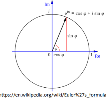
5.1.3.2. Euler’s formula
Euler’s formula is the fundamental relationship between the trigonometric functions and the complex exponential function. This can be mathematically expressed as:
![\[e^{i\theta} = cos(\theta) + i sin(\theta)\]](https://uhlibraries.pressbooks.pub/app/uploads/quicklatex/quicklatex.com-aaa27af4c253d5cd3d97d7c0a5af0932_l3.png "Rendered by QuickLaTeX.com")
From Euler’s formula, we can express the complex number as:
![\[z = rcos(\theta) + i rsin(\theta) = re^{i\theta}\]](https://uhlibraries.pressbooks.pub/app/uploads/quicklatex/quicklatex.com-1e15092524cbf5090dc54da36f7c9fd1_l3.png "Rendered by QuickLaTeX.com")
Therefore, z can also be expressed as:
![\[z = re^{i\theta}\]](https://uhlibraries.pressbooks.pub/app/uploads/quicklatex/quicklatex.com-f06f98dc1a21de3f8623b5dd89effc8a_l3.png "Rendered by QuickLaTeX.com")
Test your understanding: Euler’s Formula
Let 
Calculate 
Hint: Just plug in  to the function
Ans: i
Consider that a mathematical notation for a cosine wave is:
![\[f(t) = A.cos(\theta)\]](https://uhlibraries.pressbooks.pub/app/uploads/quicklatex/quicklatex.com-bcc1ee8b3addc91302b7e06cc27cc2f6_l3.png "Rendered by QuickLaTeX.com")
where A is the amplitude and  is phase.
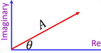
A different way to to express that wave is to use the following notation:
![\[f(t) = Ae^{i\theta}\]](https://uhlibraries.pressbooks.pub/app/uploads/quicklatex/quicklatex.com-3d8c016a467b8214ce7a47e97e8f55bb_l3.png "Rendered by QuickLaTeX.com")
The representation of this in the complex plane is as follows;
(Note that if you were to see something that looks like  , please always keep in mind that this represents sinusoidal waves with amplitude A and phase
  )
)
5.1.3.3. Deriving a complex number
Deriving an exponential function is much simpler than deriving a trigonometric function. Consider the following problem;
![\[\frac{\partial e^{i\omega t}}{\partial t} = i \omega e^{i\omega t}\]](https://uhlibraries.pressbooks.pub/app/uploads/quicklatex/quicklatex.com-bb949191a03a1ddf27a1be5e09bb9193_l3.png "Rendered by QuickLaTeX.com")
Now, remember that:
![\[i = e^{i\frac{\pi}{2}}\]](https://uhlibraries.pressbooks.pub/app/uploads/quicklatex/quicklatex.com-a5e3813bbcfb331d42c3cad51befeac1_l3.png "Rendered by QuickLaTeX.com")
Therefore:
![\[\frac{\partial e^{i\omega t}}{\partial t} = i \omega e^{i\omega t} = e^{i\frac{\pi}{2}}\omega e^{i\omega t}\]](https://uhlibraries.pressbooks.pub/app/uploads/quicklatex/quicklatex.com-203e4f30a4e0c7f73360df720042029f_l3.png "Rendered by QuickLaTeX.com")
![\[\frac{\partial e^{i\omega t}}{\partial t} = \omega e^{i(\omega t + \frac{\pi}{2})}\]](https://uhlibraries.pressbooks.pub/app/uploads/quicklatex/quicklatex.com-6460129113aadb9f95e542b2a59f78e3_l3.png "Rendered by QuickLaTeX.com")
Notice that the argument in the exponential has changed from  to
to 
The conclusion to this is that when you take a time derivative, the phase will change by  .
.
5.1.3.4. Why bother with complex numbers?
The first question that you might ask is: why do we need to know about complex numbers? The reason is: It turns out, the whole Fourier theory was built upon complex variables.
Other than that, complex numbers offers a lot of mathematical conveniences, such as:
- No need to deal with trigonometric functions
- Exponentials are easier to manipulate
- Some problems can be solved easier using complex number/complex analysis (examples: quantum physics, conformal transformations, AC circuits, etc.)
If you are interested to learn more about complex numbers, here are some resources that might be of interest:
• Complex Analysis Made Simple on youtube.
• MIT OpenCourseWare: Development of the
complex numbers
• Functions of complex variables in StackExchange
•Intuitive Arithmetic with Complex Numbers (Betterexplained.com)
5.2. Fourier transform
5.2.1. waveforms and amplitude spectrum
Virtually, any real world waveforms can be represented as a sum of sins, no matter how complicated they may look.
For example, take a look on this waveform:
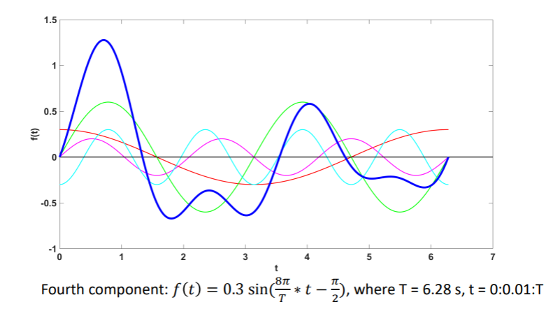
The blue waveform may look complicated, but it is actually the sum of four other sinusoidal functions in the above graph, with the equation for each line being;
Red line: 
Green line: 
Magenta line: 
Cyan line: 
This proves that no wonder how complex they are, waveforms are just a sum of sinusoidal waves.
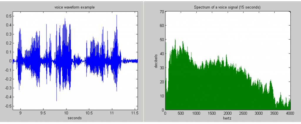
If we were to plot a waveform that is the sum of two sinusoidal waves, and plot the magnitude of each wave in terms of their frequency, we get something like this:
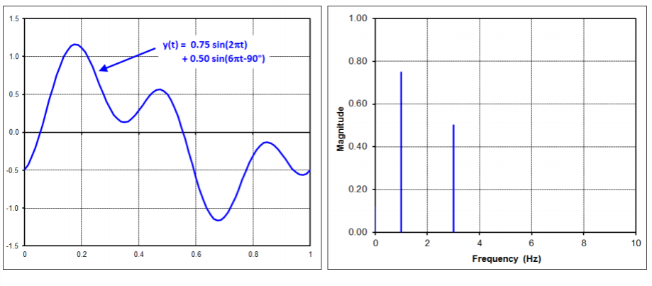
The signal results from the sum of two sine waves. These two waves have different amplitudes, frequencies, and phases, and this difference is made more clear in the amplitude spectrum on the right side of the above figure.
Another way to look at the difference between frequency domain and time domain is with the following figure:
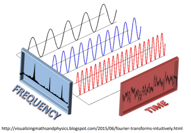
The figure above shows two different ways of viewing the combination of these 3 waveforms. In time domain, it is the summation of these three waveforms (with noise), and thus the perceived signal in the time domain looks more complicated. When viewing the three waveforms in the frequency domain, it is in the form of three separate peaks that tells you the frequency and amplitude of said waveforms.
5.2.2. definition
Mathematically speaking, any waveform function can be expressed as:
![\[f(t) = \frac{1}{2\pi} \int_{-\infty}^{\infty} F(\omega) e^{i\omega t} dw\]](https://uhlibraries.pressbooks.pub/app/uploads/quicklatex/quicklatex.com-728d4e74bf799eda28b340f8f5cfb4b8_l3.png "Rendered by QuickLaTeX.com")
The term  is a sinusoidal wave, with the amplitude being
  . This essentially says that any waveform is a sum of many sinusoidal waves with different amplitudes, phases, and frequencies.
The Fourier Transform allows us to find the constituent frequencies given a signal in time domain. This is mathematically expressed as:
![\[F(\omega) = \int_{-\infty}^{\infty} f(t) e^{-i\omega t} dt\]](https://uhlibraries.pressbooks.pub/app/uploads/quicklatex/quicklatex.com-e1140da4932c3c5fd28b70410846720b_l3.png "Rendered by QuickLaTeX.com")
It decomposes a signal into a series of sinusoidal waves of different amplitudes, frequencies, and phases. This helps identify what the sine and cosine components that make up the signal are.
The inverse Fourier transform is thus:
In terms of notation, we refer the Fourier transform of a function  as the capital
  , and the inverse Fourier transform as
  . Putting this in mathematical perspective:
Fourier Transform: ![F[f(t)] = F(\omega)](https://uhlibraries.pressbooks.pub/app/uploads/quicklatex/quicklatex.com-3724816a38f830755a6afea3563b0e60_l3.png "Rendered by QuickLaTeX.com")
Inverse Fourier Transform: ![F^{-1}[F(\omega)] = f(t)](https://uhlibraries.pressbooks.pub/app/uploads/quicklatex/quicklatex.com-1465456bce001126685cd927fe9a30e6_l3.png "Rendered by QuickLaTeX.com")
If you want to know more about Fourier transform(FT), here’s some optional reading material on FT:
- https://betterexplained.com/articles/an-interactive-guide-to-the-fourier-transform/
- http://visualizingmathsandphysics.blogspot.com/2015/06/fourier-transforms-intuitively.html
- https://www.ritchievink.com/blog/2017/04/23/understanding-the-fourier-transform-by-example/
- https://learn.adafruit.com/fft-fun-with-fourier-transforms/background
5.2.3. from time domain to spatial domain
For now, you might notice that everything that we have talked about so far is in time domain. However, potential field data is in the spatial domain. This does not seem to be a problem because Fourier transform also applies in the spatial domain. The Fourier transform in time and spatial domain can be seen in the following figure:
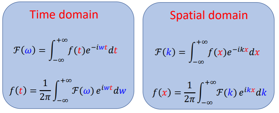
Notice that they are both the same, except for the fact that the Fourier transform of a in time(t) domain is a function of angular frequency (), and in spatial(x) domain, the Fourier transform is a function of wavenumber(k). Thus, everything in spatial domain is the same as in time domain, except we’re dealing with space (x) instead of time (t), and the Fourier transform involves wavenumber (k) instead of angular frequency ().
As we mentioned before, frequency is a measure of how many cycles per unit of time. Wavenumber is the measure of how many cycles per unit of distance. The following equation applies for wavenumber:
![\[k= \frac{2\pi }{\lambda}\]](https://uhlibraries.pressbooks.pub/app/uploads/quicklatex/quicklatex.com-27e6bc3fdbdc965b8fb89fdea4e19994_l3.png "Rendered by QuickLaTeX.com")
![\[f =\frac{1}{\lambda}\]](https://uhlibraries.pressbooks.pub/app/uploads/quicklatex/quicklatex.com-2994aab569a01438bb2320f43efcb1e4_l3.png "Rendered by QuickLaTeX.com")
Where  is the wavelength (one cycle in unit of distance).
Another concern is that the data maps that we have dealt with are 2-dimensional. Therefore, if we were to take the Fourier transform of such spatial data maps, then we need to do a 2D Fourier transform in spatial domain. The following is such equation:
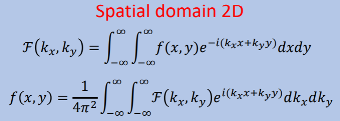
Note that  is the wavenumber in the x axis and
  is the wavenumber in the y axis respectively.
5.2.4. DC-component
There is one interesting result that we can see from the Fourier transform:
![\[F(k) = \int_{-\infty}^{\infty} f(x)e^{-ikx}\]](https://uhlibraries.pressbooks.pub/app/uploads/quicklatex/quicklatex.com-76f522fad2d63d2865e0bc542d7c2c0f_l3.png "Rendered by QuickLaTeX.com")
If we have k=0, that means the Fourier transform would be:
![\[F(0) = \int_{-\infty}^{\infty} f(x)e^{-i.0.x} = \int_{-\infty}^{\infty} f(x) dx\]](https://uhlibraries.pressbooks.pub/app/uploads/quicklatex/quicklatex.com-14a5b5a1d526a2fa14331ef2be77a65e_l3.png "Rendered by QuickLaTeX.com")
Fourier transform of a function f(x) evaluated at k=0 is simply the integral of this function over the entire x axis. And it is always real if f(x) is real. We call this the DC Component. Thus, the DC component is the Fourier transform of a function f(x) evaluated at k=0.
5.2.5. Amplitude and phase
In general, Fourier transform of  is a complex function with a real and an imaginary part:
![\[F(k) = Re(F(k)) + i Im(F(k))\]](https://uhlibraries.pressbooks.pub/app/uploads/quicklatex/quicklatex.com-7b2da029b7f832be9a4ccff3d7f77c52_l3.png "Rendered by QuickLaTeX.com")
Which also can be written as:
![\[F(k) = |F(k)|e^{i\theta(k)}\]](https://uhlibraries.pressbooks.pub/app/uploads/quicklatex/quicklatex.com-90cf1424f59a750fc5dfb64c187cf55d_l3.png "Rendered by QuickLaTeX.com")
where:
![\[|F(k)| = \sqrt(Re(F(k))^2 + (Im(F(k)))^2)\]](https://uhlibraries.pressbooks.pub/app/uploads/quicklatex/quicklatex.com-f6e309a850a7a1097577da5ddb499612_l3.png "Rendered by QuickLaTeX.com")
and
![\[\theta(k) = arctan\frac{Im(F(k))}{Re(F(k))}\]](https://uhlibraries.pressbooks.pub/app/uploads/quicklatex/quicklatex.com-9fac81ba1dae46f10257b79edc30df57_l3.png "Rendered by QuickLaTeX.com")
5.2.6. properties
There are several properties of Fourier transform. We will cover each one in this section.
5.2.6.1. Linearity
If we have a two functions in the spatial domain, with each having a Fourier transform:


Then the summation of the two functions in the spatial domain is also the summation in the Fourier domain as such:
![\[a_1f_1(x) + a_2f_2(x) \leftrightarrow a_1F_1(k)+a_2F_2(k)\]](https://uhlibraries.pressbooks.pub/app/uploads/quicklatex/quicklatex.com-07df10328cf378ad77707d2989a278d9_l3.png "Rendered by QuickLaTeX.com")
5.2.6.2. Scaling
If we have a function  with its Fourier transform :
  , then if you stretch your by 0.5, we would have an with narrower band and higher amplitude. This is mathematically expressed as:
![\[f(ax) \leftrightarrow \frac{1}{|a|} F(\frac{k}{a})\]](https://uhlibraries.pressbooks.pub/app/uploads/quicklatex/quicklatex.com-096b83d6fc9572087304242b7ddcbebb_l3.png "Rendered by QuickLaTeX.com")
- If a>1, we shrink the signal (the signal contains more high frequency content), then the Fourier transform of this new signal will contain higher frequencies (hence the
 )
) - If a<1, we stretch the signal (the signal contains more low-frequency contents) then the Fourier transform of this new signal will contain lower frequencies
An example of this property can be seen in the following graph.
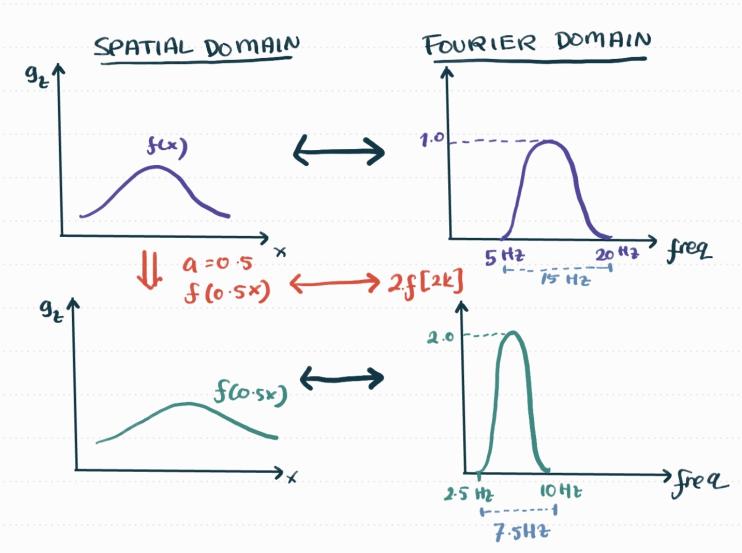
Thus, a broad anomaly will have a narrower amplitude spectrum than a narrow anomaly. Because the width of an anomaly is directly related to the depth of its source, we can expect that the narrowness of a Fourier-transformed anomaly will also be related to the depth of the source.
Scaling Property
If you stretch in spatial domain  you are shrinking in Fourier domain
If you shrink in spatial domain you are stretching in Fourier domain
5.2.6.3. Shifting
If you have a function such that , then:
![\[f(x-x_0) \leftrightarrow F(k)e^{-ikx_0}\]](https://uhlibraries.pressbooks.pub/app/uploads/quicklatex/quicklatex.com-b197e1a7235794071d01a580ec980a8f_l3.png "Rendered by QuickLaTeX.com")
Shifting a function along the x axis in the spatial domain is equivalent to adding a linear phase factor to the function’s Fourier transform. The amplitude spectrum is unaffected.
5.2.6.4. Differentiation
If we have a function such that: 
then:
![\[\frac{d}{dx} f(x) \leftrightarrow ikF(k)\]](https://uhlibraries.pressbooks.pub/app/uploads/quicklatex/quicklatex.com-b313c8bb91eb82eb2da77b052c496010_l3.png "Rendered by QuickLaTeX.com")
As mentioned before in the previous section, the phase will change by . Thus, the amplitudes for low-frequency components will be suppressed, and the amplitudes for high-frequency components will be amplified.
The concept of differentiation in the Fourier domain is applied in potential field data. Specifically, for derivative-based anomaly enhancement. For example, the following figure shows a bouguer anomaly and Gzz data map. We can see that by taking the derivative of the gravity data, the anomalies are more enhanced and thus we see the boundaries of the anomaly clearer.
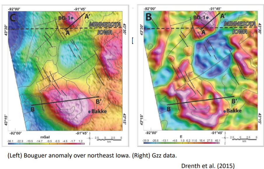
Another way to enhance the anomaly is to take the horizontal gradient of the magnitude as seen in the following picture. We can see that the boundaries are more accentuated in the data map on the right.
Bouguer anomaly
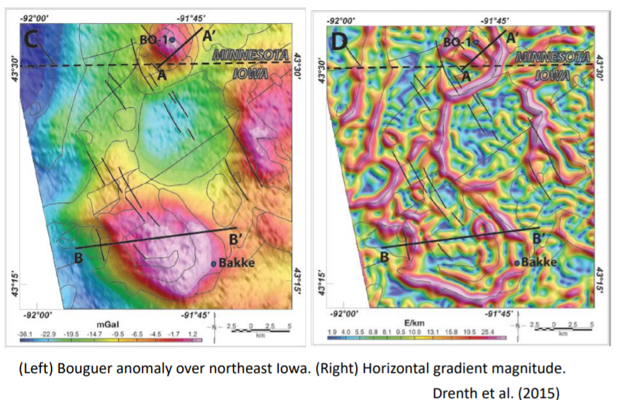
Tensor data
With how well derivatives are in enhancing the anomalies, it is no surprise that we would want to do Fourier transform to these data maps. This is because, as mentioned before, the math involved in derivation in the fourier domain is much more simpler than in spatial domain.
Summary of Fourier Transform Properties
The properties of Fourier transform are:
- Linearity: Suppose that and , then:
- Scaling: Suppose that , then:
- Shifting: Suppose that , then:
- Differentiation: Suppose that , then:
5.2.6.5. Fourier transform of 1/r
If you still remember the gravity potential, the equation is shown:
![\[U(p)=\gamma\frac{dm}r\]](https://uhlibraries.pressbooks.pub/app/uploads/quicklatex/quicklatex.com-210fc089f1639bbfddb38f5c2d07eb2f_l3.png "Rendered by QuickLaTeX.com")
where  is the gravitational constant,
  is a small mass over the
  .
.
Similar to the magnetic scalar potential:
![\[V(p)=\frac{\mu_0}{4\mathrm\pi}\frac{\mathbf{m}\cdot\widehat{ \mathbf{r}}}{r^2}=-\frac{\mu_0}{4\mathrm\pi}\mathbf{m}\cdot\nabla_p\frac1r\]](https://uhlibraries.pressbooks.pub/app/uploads/quicklatex/quicklatex.com-515e46e262dacd653d39a1a35a9be81a_l3.png "Rendered by QuickLaTeX.com")
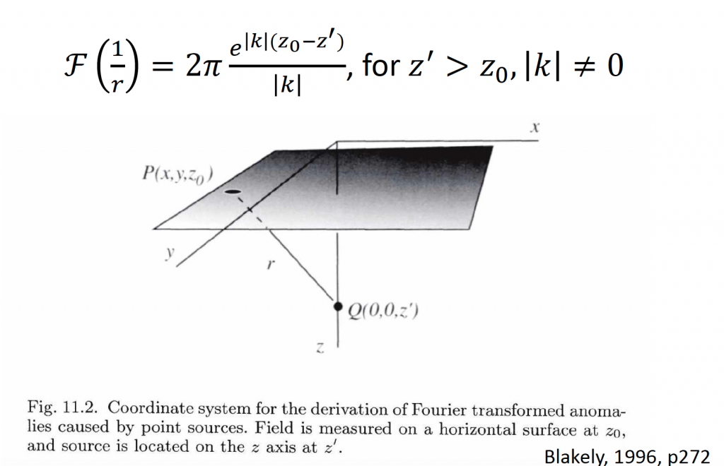
We observe that both gravity potential and magnetic scalar potential have the  . Before we apply Fourier transform to gravity potential and magnetic scalar potential, we need to figure out the Fourier transform of . Specifically, we need to make use of Bessel function and Hankel transform. But the derivation is mathematically involved, so we will skip the detailed derivations. For those who are interested, please refer to Blakely (1996, p271-273).
After a series complicated derivation, we obtain:
![\[\mathcal F(\frac1r)=2\mathrm\pi\frac{\mathrm e^{\left|\mathrm k\right| ({\mathrm z}_0-\mathrm z^{'})}} {\left|\mathrm k\right|}\]](https://uhlibraries.pressbooks.pub/app/uploads/quicklatex/quicklatex.com-0c71368d7b1d648aa73aea11b43a1696_l3.png "Rendered by QuickLaTeX.com")
where,  >
> ,
,  ,
,  is wave number.
The equation above is the results for Fourier transform of .
5.3. Terminology
5.3.1. Amplitude and phase, amplitude sepctrum and phase spectrum
We can use an equation to do Fourier transform (shown in below).
![\[\mathcal F(k)=\int_{-\infty}^{+\infty}{f(x)e^{-ikx}}\operatorname dx\]](https://uhlibraries.pressbooks.pub/app/uploads/quicklatex/quicklatex.com-36ed2e4d5b58914b1080e7eedb35f927_l3.png "Rendered by QuickLaTeX.com")
where is a signal. IN most general cases, Fourier transform is a complex function with a real and an imaginary part.
![\[\mathcal F(k)=Re\mathcal F(k)+iIm\mathcal F(k)\]](https://uhlibraries.pressbooks.pub/app/uploads/quicklatex/quicklatex.com-d61f96f46da8f402e744a3d28d5da8ee_l3.png "Rendered by QuickLaTeX.com")
Also, if we apply Euler’s formulation, the Fourier transform can be expresses as:
![\[\mathcal F(k)=\left|\mathcal F(k)\right|e^{i\Theta(k)}\]](https://uhlibraries.pressbooks.pub/app/uploads/quicklatex/quicklatex.com-d1d7fd69bd2509e9df4dc6a62ff603da_l3.png "Rendered by QuickLaTeX.com")
where,
![\[\left|\mathcal F(k)\right|=\sqrt{(Re\mathcal F{(k))}^2+(Im\mathcal F{(k))}^2}\]](https://uhlibraries.pressbooks.pub/app/uploads/quicklatex/quicklatex.com-a746d4e86ccee00a43853004cf829ab9_l3.png "Rendered by QuickLaTeX.com")
![\[\Theta(k)=arc\tan\frac{Im\mathcal F{(k)}}{Re\mathcal F(k)}\]](https://uhlibraries.pressbooks.pub/app/uploads/quicklatex/quicklatex.com-e6eacf7e2a395e56bb518597435601a2_l3.png "Rendered by QuickLaTeX.com")
The  is called amplitude and
  is named phase. If we want to transform a signal from spatial domain to the Fourier domain, we need to know both amplitude and phase.
is simply called amplitude spectrum, which is a function of wave number . In similar, we also called phase spectrum, which means how phase change with the wave number .
5.3.2. Energy and power spectrum
The total energy of a real function f(x). It is an integral of entire real axis of the square of amplitude, which measures how much energy in function  .
.
![\[E=\int_{-\infty}^{+\infty}\left|\mathcal F(k)\right|^2\operatorname dk\]](https://uhlibraries.pressbooks.pub/app/uploads/quicklatex/quicklatex.com-991cbc14701c4ca92298903cbe807dca_l3.png "Rendered by QuickLaTeX.com")
where is Fourier transform which is a complex number.  is also called energy density function over frequency, which tells us, how energy of this function distribute with different wave numbers over frequency band. Sometimes, is named energy spectral density, power spectral density (PSD) or power spectrum (PS).
We can see some high amplitude and low amplitude in the figure above (left), if we do the integration of square of amplitude, we will obtain the power spectrum (right).
5.4. Gravity foR a point mass in Fourier domain
Recall Fourier transform of 1/r

Based on the Fourier transform of 1/r, we can calculate the 3D gravity modeling in Fourier domain with point mass.
![\[U=\gamma\frac\mu r\]](https://uhlibraries.pressbooks.pub/app/uploads/quicklatex/quicklatex.com-5db40adc1963af799d42fc0b69c27010_l3.png "Rendered by QuickLaTeX.com")
where  is point mass, U is gravitational potential. Then we apply Fourier transform, and will obtain:
![\[\mathcal F(U)=\mathcal F(\gamma\frac\mu r)=\gamma\mu\mathcal F(\frac1r)\]](https://uhlibraries.pressbooks.pub/app/uploads/quicklatex/quicklatex.com-6307cf2690e4e36a83a89146dd05a8c8_l3.png "Rendered by QuickLaTeX.com")
After applying Fourier transform of 1/r, it is easily to get:
![\[\mathcal F(U)=2\mathrm\pi\gamma\mu\frac{\mathrm e^{\left|\mathrm k\right| ({\mathrm z}_0-\mathrm z^{'})}} {\left|\mathrm k\right|}\]](https://uhlibraries.pressbooks.pub/app/uploads/quicklatex/quicklatex.com-91b81c4546f8dc0df5f0b6b4e48f49ab_l3.png "Rendered by QuickLaTeX.com")
where, >, .
We currently measures the vertical component of gravity field Gz, which is derivative of gravity potential in z direction.
![\[g_z=\frac{\partial U}{\partial z}=\gamma\mu\frac{\partial{}}{\partial z}\frac1r\]](https://uhlibraries.pressbooks.pub/app/uploads/quicklatex/quicklatex.com-563e4b4f88e938a9249a9159a88c7caa_l3.png "Rendered by QuickLaTeX.com")
Then, we apply Fourier transform,
![\[\mathcal F(g_z)=\mathcal F(\gamma\mu\frac\partial{\partial z}\frac1r)=\gamma\mu\mathcal F(\frac\partial{\partial z}\frac1r)\]](https://uhlibraries.pressbooks.pub/app/uploads/quicklatex/quicklatex.com-694b950922e75104293f952facc4bd79_l3.png "Rendered by QuickLaTeX.com")
The derivative in z direction has nothing to do in x, y direction, so we can directly take the derivative outside, and obtain the following equation:
![\[\mathcal F(g_z)=\gamma\mu\frac\partial{\partial z}\mathcal F(\frac1r)=2\mathrm \pi \gamma\mu e^{\left|\mathrm k\right|({\mathrm z}_0-\mathrm z^{'})}\]](https://uhlibraries.pressbooks.pub/app/uploads/quicklatex/quicklatex.com-2c274755b585a4e510d1910a5bbc89ad_l3.png "Rendered by QuickLaTeX.com")
Thus, we obtain the gravity measure (z component) after Fourier transform:
![\[\mathcal F(g_z)=2\mathrm \pi \gamma\mu e^{\left| \mathrm k\right|({z}_0- z^{'})}\]](https://uhlibraries.pressbooks.pub/app/uploads/quicklatex/quicklatex.com-2ec61e6404d21377aa1dd3db7d1f2c9e_l3.png "Rendered by QuickLaTeX.com")
Next, we are going to make a few observations about the equation, which will help us better understand the gravity.
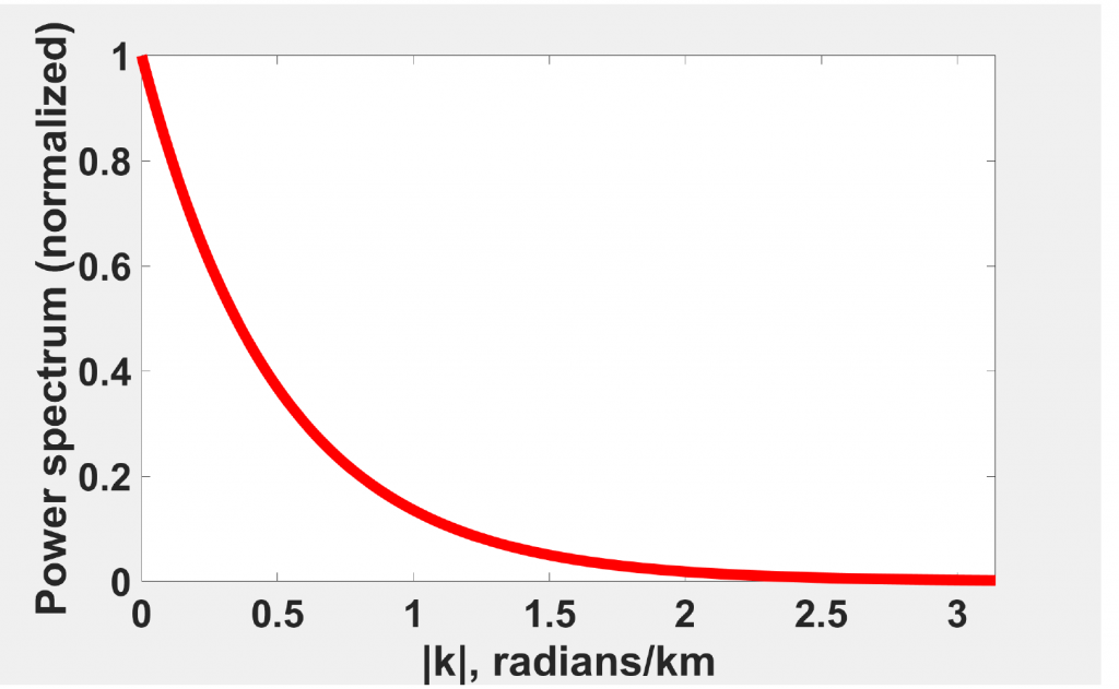
The x axis is wave number, y axis is normalized power spectrum of gravity anomalies with a point mass. This figure thus tell us how much energy there is at each wavenumber. The most obvious thing here is exponential decay. Another observation is maximum energy occurs at k=0 (zero wavenumber). When k = 0, we can obtain:
![\[\mathcal F(g_z)=2\mathrm \pi \gamma\mu\]](https://uhlibraries.pressbooks.pub/app/uploads/quicklatex/quicklatex.com-f75313639e3c2692d2b46fb7661fd42b_l3.png "Rendered by QuickLaTeX.com")
where, is a constant value, is mass.
We can easily observe that the power spectrum value at k=0 is proportional to the total mass.
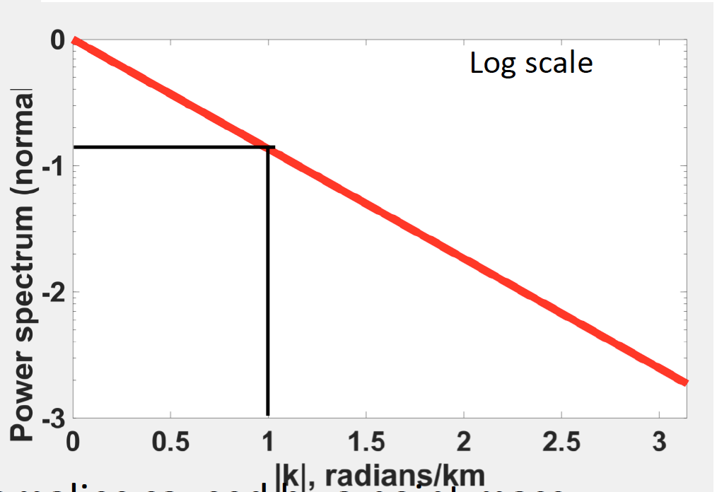
Observation from the power spectrum in log scale, we noticed that it is a straight line with negative slope. Besides, the energy decreases exponentially with increasing wavenumber. The black lines show that the x axis is 1, y axis is -1, so the slope is -1. We knew that the depth is negative slope, so the depth for the anomaly in the figure above is 1 m.
The rate of decreases on log scale is equal to the elevation difference between the source body and observation plane.
![\[\log(\mathcal F(g_z))=\log(2\mathrm{πγμ})+\left|k\right|(z_0-z^{'})\]](https://uhlibraries.pressbooks.pub/app/uploads/quicklatex/quicklatex.com-35e1b7fa8e49fdb4a09ed17b60ff8410_l3.png "Rendered by QuickLaTeX.com")
If we set  ,
,
![\[\log(\mathcal F(g_z))=\log(2\mathrm{πγμ})+\left|k\right|h\]](https://uhlibraries.pressbooks.pub/app/uploads/quicklatex/quicklatex.com-addbcaf23e3d68581ffc7d2d22b493ed_l3.png "Rendered by QuickLaTeX.com")
The equation above mathematically illustrates that the rate of decrease depends on the depth of the source body.
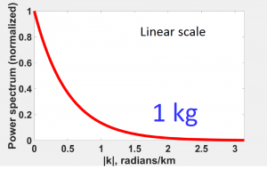
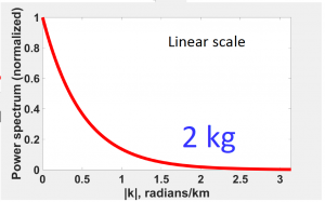
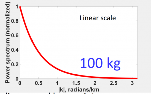
The figures above have same depth but different masses, we noticed the trend is completely same, which means the mass does not change the decay rate and the decay rate has only to do with h.
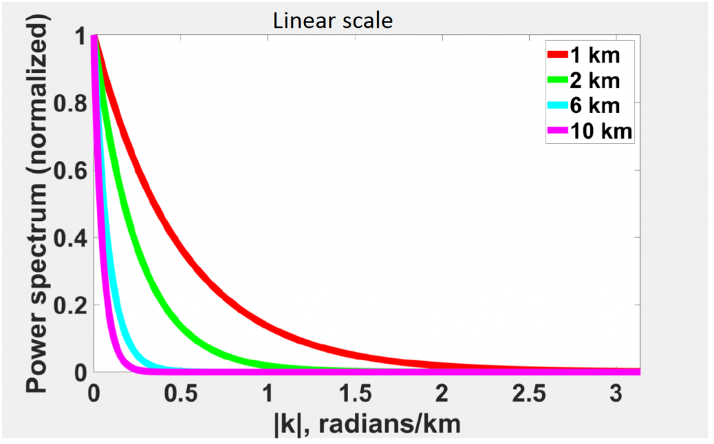
Here we created a synthetic model with same mass but located in different depth. The red line is shallowest one. We noticed from the figure above is if the source body is deeper, the energy decay faster and faster. Specifically, look at the source body located at 10 km, the energy decay to 0 at 0.2 radians/km. In comparison, if source body located at 2 km (green) line, the energy decays to 0 when wavenumber is about 1.2 radians/km.
Then, we plot 4 cases in log scale, shown in below:
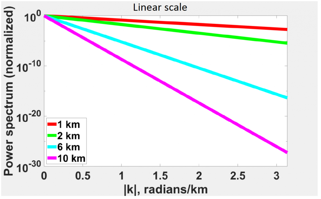
In similar trend, the source body is deeper, the energy decay is faster and faster, where energy decay is represented by the slope. The slope equal to -h, so the slope is smaller, the depth is deeper and the energy decay is faster.
The summaries of two figures above
- The decay rate depends upon depth.
- The deeper the source, the faster the energy decays.
- As source become deeper, energy at higher – wave numbers become smaller.
- The gravity anomaly is approximately band limited.
In previous experiment, we fixed observation at 0 km, and varied the depth of source bodies: 1km, 2km, 6 km and 10 km. If we fix the source body at a depth of 1 km and change the observation height: 0km, -1 km, -5 km, and -9km, we will observe the exact same thing (shown in the figure below).
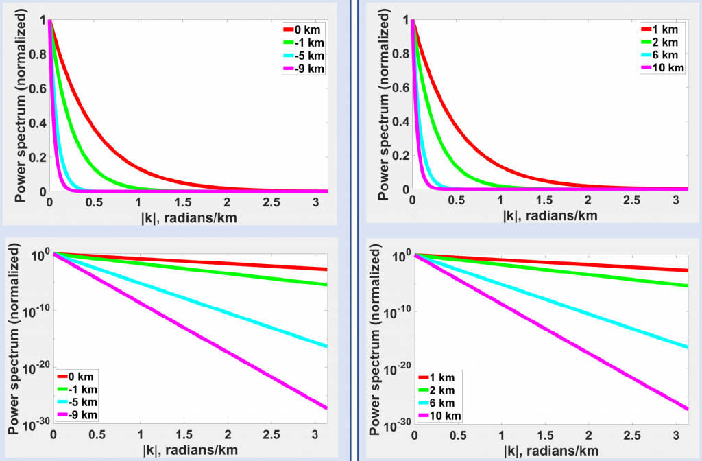
From the figure above (top left and bottom left), we noticed that when source depth fixed, the decay rate depends upon observation height. The higher the observation height, the faster the energy decays. As observation become higher, energy at higher, wave numbers become smaller.
This observation plays a critical role in data acquisition that is: if you want to resolve fine details (i.e., high wave number information) of your targets, you need to be closer to your target. If using the airborne platform, we have to fly as lower as we can.
Here are several examples.
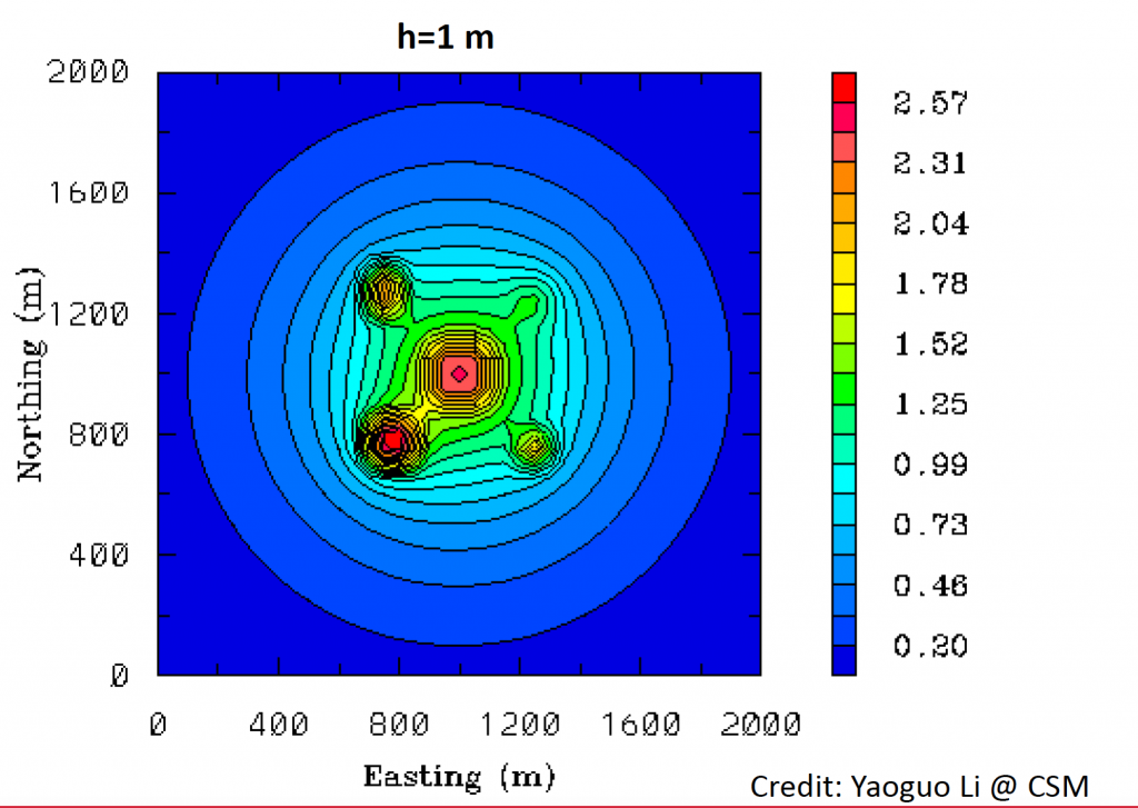
This is one field gravity data map simulated from five source bodies with fixed depth. The data map shown above is 1 meter above the surface. We can easily see the features at data maps.
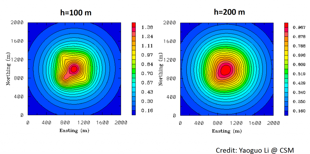
In the top right figure, we keep source body shape, depth same and the only thing changed is observation height. The observation height is changed from 1 m to 100 m. Compared with previous map, we noticed that anomalies become much smooth. But we can still see a few features of source body. We can still tell there something subsurface. Keeping increasing observation height to 200 m, this map is smooth and it is always explained as one source body rather five.
The observation from the above figures is the height is higher, the gravity anomalies become smoother that means less high frequency information. This phenomenon can be explained as the higher the observation height, the faster the energy decays and wave numbers become smaller.
Another example is:
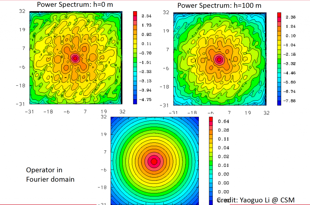
From the figure above, we noticed that the height of observation is increased, the power spectrum becomes more smooth. The more details about the figures above will be discussed in the following sections.
A quick summary
- We have made quite a few observations based on this simple equation.
- These insights help understand gravity well.
- This is one of the reasons why we look at gravity data in Fourier doamin.
5.5. FOURIER DOMAIN MODELING OF MAGNETIC DATA DUE TO A DIPOLE
Let’s move on to the magnetic data for the simplest case of considering a magnetic dipole.
5.5.1. Fourier transform of magnetic potential
For the magnetic scalar potential  , which is the dot product of two vectors expressed in the following equation:

Where the dipole moment is expressed as its magnitude and directions in 3D by ![\mathbf{m}=m{{[{{\hat{m}}_{x}},{{\hat{m}}_{y}},{{\hat{m}}_{z}}]}^{T}}](https://uhlibraries.pressbooks.pub/app/uploads/quicklatex/quicklatex.com-c568842d18adc2d1560b9cae31db5753_l3.png "Rendered by QuickLaTeX.com") .
.
According to the definition of the dot product, the above magnetic scalar potential expression can be rearranged into the following equation:

If we apply the Fourier transform to the magnetic potential in the above equation, through using properties such as the linearity and differentiation, we will then have the derivations as shown below. Since we are taking the Fourier transform in 2D x-y domain, the z-direction differentiation is not relevant here.
![F\left[ V \right]=-\frac{{{\mu }_{0}}}{4\pi }m\cdot \left( {{{\hat{m}}}_{x}}i{{k}_{x}}F\left[ \frac{1}{r} \right]+{{{\hat{m}}}_{y}}i{{k}_{y}}F\left[ \frac{1}{r} \right]+{{{\hat{m}}}_{z}}\frac{\partial }{\partial z}F\left[ \frac{1}{r} \right] \right)](https://uhlibraries.pressbooks.pub/app/uploads/quicklatex/quicklatex.com-714a9eadbc3d46e28a6da27b4b6406b6_l3.png "Rendered by QuickLaTeX.com")
After above derivation, we are left with familiar expression of ![F\left[ \frac{1}{r} \right]](https://uhlibraries.pressbooks.pub/app/uploads/quicklatex/quicklatex.com-6db10855458932c3de7d03bfce18dc61_l3.png "Rendered by QuickLaTeX.com") , which equals
, which equals  , with z’ > z0.
Therefore, after substituting it into the Fourier transform equation, the simplified expression for the Fourier transform of magnetic potential is as following, consisting of four parts, the constant number  , the magnitude of dipole moment
  , the complex number
  , and the exponential expression
  which only depends on the source body depth.
![F\left[ V \right]=-\frac{{{\mu }_{0}}}{2}m{{\Theta }_{m}}{{e}^{\left| k \right|\left( {{z}_{0}}-{{z}^{'}} \right)}}](https://uhlibraries.pressbooks.pub/app/uploads/quicklatex/quicklatex.com-c56418cbf9fdc97c2d1ebdbb8b54631f_l3.png "Rendered by QuickLaTeX.com")
Where the complex number

depends only on the orientation of the dipole.
5.5.2. Fourier transform of total-field anomaly
Practically in the field survey, most likely we will collect total-field anomaly  as the magnetic data. Therefore, we can derive the vector B field by taking the negative gradient of the potential V, which can be mathematically expressed as:

That is, any component (such as  ) can be derived from the directional derivative of the magnetic potential.
As we have talked before, the total field anomaly is simply the projection of the Bfield onto the inducing field direction, which is ![\mathbf{\hat{f}}={{\left[ {{{\hat{f}}}_{x}},{{{\hat{f}}}_{y}},{{{\hat{f}}}_{z}} \right]}^{T}}](https://uhlibraries.pressbooks.pub/app/uploads/quicklatex/quicklatex.com-9a0bdadefd02e7c2f11a3f7575175336_l3.png "Rendered by QuickLaTeX.com") . Therefore, mathematically, the total field anomaly is equal to the dot product of the inducing field direction with the Bfield, as shown below:
. Therefore, mathematically, the total field anomaly is equal to the dot product of the inducing field direction with the Bfield, as shown below:

Similarly, after applying the Fourier transform to the total field anomaly, we will get the expression as follows:
![\mathbf{F}\left[ \Delta T \right]=-{{{\hat{f}}}_{x}}i{{k}_{x}}\mathbf{F}\left[ V \right]-{{{\hat{f}}}_{y}}i{{k}_{y}}\mathbf{F}\left[ V \right]-{{{\hat{f}}}_{z}}\frac{\partial }{\partial z}\mathbf{F}\left[ V \right]](https://uhlibraries.pressbooks.pub/app/uploads/quicklatex/quicklatex.com-661a44bb8d2bbe5bcf619657005b4026_l3.png "Rendered by QuickLaTeX.com")
After simplifying this expression, we will have the Fourier transform as shown below, which consists of four parts: the constant number, the magnitude of dipole moment (i.e., it depends on the source strength), the two directional dependent complex numbers and , and the depth-relevant exponential expression .
![\mathbf{F}\left[ \Delta T \right]=\frac{{{\mu }_{0}}}{2}m{{\Theta }_{m}}{{\Theta }_{f}}\left| k \right|{{e}^{\left| k \right|\left( {{z}_{0}}-{{z}^{'}} \right)}}](https://uhlibraries.pressbooks.pub/app/uploads/quicklatex/quicklatex.com-dfbce84b540b10f4eb8ba930b2b484ba_l3.png "Rendered by QuickLaTeX.com")
Where another complex number is  , and it depends only on inducing field direction;
And the complex number depends only on the orientation of the dipole.
5.5.3. Fourier transform of total-field anomaly in polar coordinates
In order to better understand the Fourier transform of the total field anomaly expression derived above, let’s introduce its representation in polar system.
In the formulas of the complex number ,
it consists of  and
and  , which are wavenumbers in x and y directions. If we express and in polar coordinates, graphically explained in the figure below, we will have:
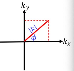


where  is the radial wavenumber.
After replacing the and in polar coordinates, the can then be written as:

Another way of representing is by using the Euler’s formula through amplitude and phase as a function of the angle , which can be re-written as

Similarly, we can follow the same procedure to represent , which we will get:

Now, let us substitute the polar representations of and into the Fourier transform expression of the total field anomaly, we will get the following expression:
![\mathbf{F}\left[ \Delta T \right]=\frac{{{\mu }_{0}}}{2}m{{A}_{m}}\left( \phi \right){{e}^{i{{P}_{m}}\left( \phi \right)}} {{A}_{f}}\left( \phi \right){{e}^{i{{P}_{f}}\left( \phi \right)}}\left| k \right|{{e}^{\left| k \right|\left( {{z}_{0}}-{{z}^{'}} \right)}}](https://uhlibraries.pressbooks.pub/app/uploads/quicklatex/quicklatex.com-a5d3f63644c7b08436ac203ab347322c_l3.png "Rendered by QuickLaTeX.com")
5.5.3.1. Interpretations of the first part of the amplitude spectrum
If we only focus on the amplitude spectrum term in the above expression, which is a function of wavenumber and angle as shown below:
![\mathbf{F}\left[ \Delta T \right]=\frac{{{\mu }_{0}}}{2}m{{A}_{m}}\left( \phi \right){{A}_{f}}\left( \phi \right)\left| k \right|{{e}^{\left| k \right|\left( {{z}_{0}}-{{z}^{'}} \right)}}](https://uhlibraries.pressbooks.pub/app/uploads/quicklatex/quicklatex.com-4b71f172b22a00d308c1de41e4cd55c1_l3.png "Rendered by QuickLaTeX.com")
The first part of this amplitude spectrum  only varies with the angle , since once we fix the strength of the source body the magnitude will become a constant. Therefore, given a fixed angle , along any ray originating from the origin, this part of the amplitude spectrum value is constant, that is, there is no decay on the ray since all values on this ray are equal.
Thus, we can express the first part as  :
:

In brief summary so far, the amplitude spectrumterm can be written as:

5.5.3.2. Interpretations of the second part of the amplitude spectrum
Now let us focus on the second part of the amplitude spectrumterm  , which has nothing to do with angle , but it is related with the observation height
  and the depth
  , and the radial wavenumber
  . Then how does it look like?
The graph plotted below is what it looks like as a function of the radial wavenumber . This figure implies that the energy increases to a peak value along with the increase of the wavenumber before starting decreasing.
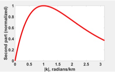
Therefore, this second part of the amplitude spectrum determines how the amplitude spectrum changes along a ray and determines the shape of the energy change in that ray.
Moreover, since this part has nothing to do with angle , the shape of the amplitude spectrum along any ray is the same; and this shape is determined by the depth of the source body .
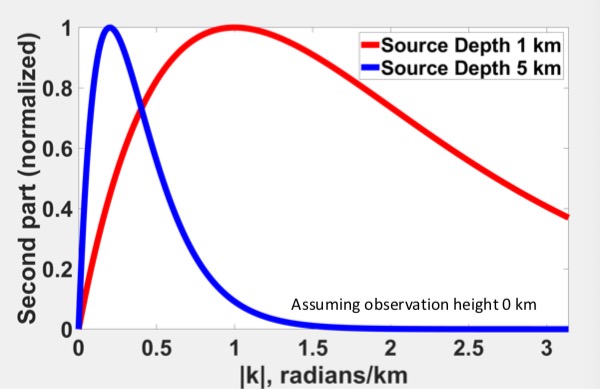
Therefore, by looking at the shape of the amplitude spectrum along any ray, we can infer depth of the source body, no matter which ray we are looking at, since they all have the exact same shapes!
In addition, the maximum energy does not occur at wavenumber k=0, but at a larger radial wavenumber that is dependent on the depth of the source dipole; once the wavenumbers exceeding this peak energy wavenumber, energy starts decaying monotonically and approaching exponential decay at higher wavenumbers.
5.6. Upward continuation
5.6.1. Concepts of upward continuation
Upward continuation is the process of using originally observed data to calculate the gravity or magnetic anomaly response that would be observed at locations above the original observation surface. Shifting the observation location to a higher elevation removes high-frequency signals from the near surface due to signal attenuation with distance. This allows for the focus of lower-frequency signals from deeper parts of a survey.
5.6.2. Upward continuation in spatial domain
Recall Green’s third identity:
![\[V\left( P \right)=\frac{1}{4\pi }\iint\limits_{Surf}{\left( \frac{1}{r}\frac{\partial V}{\partial \mathbf{\hat{n}}}-V\frac{\partial }{\partial \mathbf{\hat{n}}}\frac{1}{r} \right)}dS\]](https://uhlibraries.pressbooks.pub/app/uploads/quicklatex/quicklatex.com-54d89ee0374f591ad1b76c5de43ce14b_l3.png "Rendered by QuickLaTeX.com")
We previously stated that this is the theoretical basis for the upward continuation and the equivalent source technique. If we consider  to be harmonic, Green’s third identity is a representation formula which a potential field can be calculated at any point simply from the behavior of the field at its boundaries. This also means that no knowledge of the sources is required, except that none are located within the region. Unfortunately, the equation above requires not only the values of on the surface, but also the values of its vertical derivative. These values are unlikely to be available in most practical applications. Fortunately, through some mathematical manipulation we can eliminate the derivative from the equation, but it is fairly complex so we won’t show that here.
Eventually, we will obtain the following equation:
![\[V(x,y,z_0 - \Delta z) = \frac{\Delta z}{2\pi}\int\limits_{-\infty}^{\infty}\int\limits_{-\infty}^{\infty}\frac{V(x',y',z_0)}{[(x-x')^2 + (y-y')^2 + \Delta z^2]^{3/2}}dx'dy'\]](https://uhlibraries.pressbooks.pub/app/uploads/quicklatex/quicklatex.com-c95410c72d46d36ad764e36125800579_l3.png "Rendered by QuickLaTeX.com")

This equation is the upward-continuation integral. It shows how to calculate the value of a potential field at any point above a level, horizontal surface at from a complete knowledge of the field on the surface. This means upward continuation can be done in the spatial domain using this integral.
At this point, we will need to cover convolution. The convolution of two functions and  is:
is:
![\[h(x) = \int\limits_{-\infty}^{\infty} f(x')g(x-x')dx'\]](https://uhlibraries.pressbooks.pub/app/uploads/quicklatex/quicklatex.com-0c506d3da7c507932b78fce3bb75821e_l3.png "Rendered by QuickLaTeX.com")
We can also convert this equation to the Fourier domain if we assume that  and
and  :
:
![\[H(k) = F(k)G(k)\]](https://uhlibraries.pressbooks.pub/app/uploads/quicklatex/quicklatex.com-6c9d7a306401fe6bf2e86c47e79a6718_l3.png "Rendered by QuickLaTeX.com")
We will also need to examine convolution in 2D for upward continuation. In 2D, the convolution of two functions f(x) and g(x) in the spatial domain becomes:
![\[h(x,y) = \int\limits_{-\infty}^{\infty} \int\limits_{-\infty}^{\infty} f(x',y')g(x-x',y-y')dx'dy'\]](https://uhlibraries.pressbooks.pub/app/uploads/quicklatex/quicklatex.com-f7dfe6b62ea8d7806a15d94fa366b0df_l3.png "Rendered by QuickLaTeX.com")
If we assume that  and
and  , the Fourier domain equation is:
![\[H(k_x,k_y) = F(k_x,k_y)G(k_x,k_y)\]](https://uhlibraries.pressbooks.pub/app/uploads/quicklatex/quicklatex.com-07e90823289320ff9bf7989fbc82c782_l3.png "Rendered by QuickLaTeX.com")
This is important as we go back to our previously established upward continuation equation:
We can define
![\[\psi(x,y,\Delta z) = \frac{\Delta z}{2\pi}\frac{1}{[x^2 + y^2 + \Delta z^2]^{3/2}}\]](https://uhlibraries.pressbooks.pub/app/uploads/quicklatex/quicklatex.com-3730124feb4c6eb5238d3416bb4f0b03_l3.png "Rendered by QuickLaTeX.com")
to obtain the following equation:
![\[V(x,y,z_0 - \Delta z) = \int\limits_{-\infty}^{\infty}\int\limits_{-\infty}^{\infty}V(x',y',z_0)\psi(x-x',y-y',\Delta z)dx'dy'\]](https://uhlibraries.pressbooks.pub/app/uploads/quicklatex/quicklatex.com-2eebfaded2e71110e4718f6dac93c519_l3.png "Rendered by QuickLaTeX.com")
This equation is 2D convolution!
5.6.3. upward continuation in fourier domain
We can find the Fourier representation of upward continuation using the following equation:
![\[F[V_U] = F[V]F[\psi]\]](https://uhlibraries.pressbooks.pub/app/uploads/quicklatex/quicklatex.com-ed9384af5f9aaa52d6a68f640b49fc0b_l3.png "Rendered by QuickLaTeX.com")
All we need now is an analytical expression of F[\psi], and we will skip the derivations here to get the following equation:
![\[F[\psi] = e^{-\Delta z |k|}\]](https://uhlibraries.pressbooks.pub/app/uploads/quicklatex/quicklatex.com-d00dde687bb27c8afc56401800d290cd_l3.png "Rendered by QuickLaTeX.com")
At this point, we can find the Fourier transform of the upward-continued field in three steps:
- Transform the observed data via FFT (Fast Fourier Transform)
- Multiply by the exponential operator (e^{-h\sqrt{w_x^2 + w_y^2}})
- Apply the inverse transform to obtain the upward-continued field
5.6.4. Example
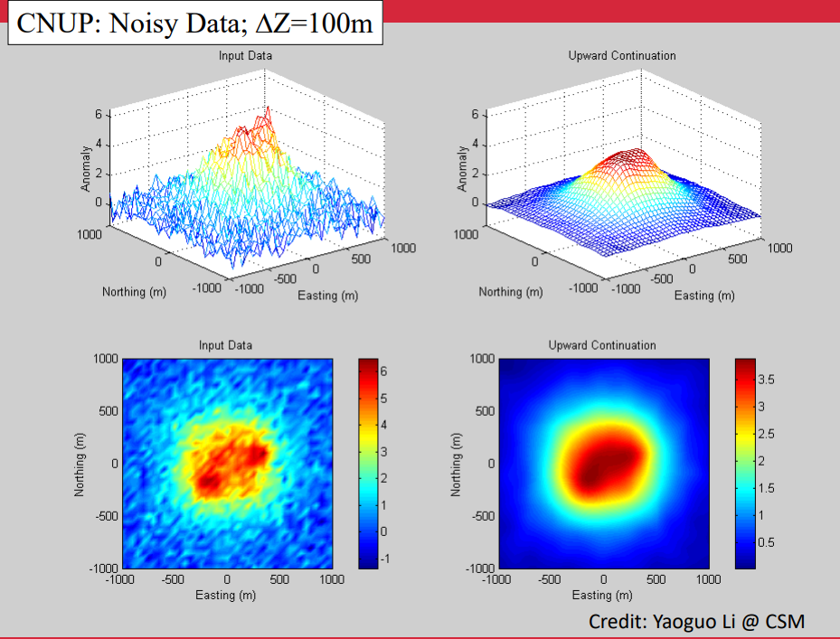
In the example below, we will be showing the influence that upward continuation has on clean and noisy data. The figure below shows the difference between the shape of the input data in 2D and 3D between its original elevation and its upward continuation.
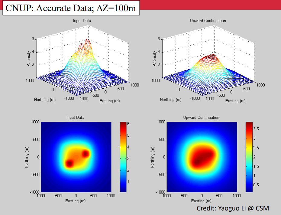
The following figure shows the same figures after noise has been introduced to the data. It is clear that the noise has a significant influence on the input data at its original data, but has been largely reduced by the upward continuation.
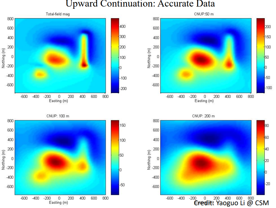
The figure below shows the magnetic response of the input data at various elevations. Pay attention to the smoothing of the overall feature along with the reduction in high-frequency data as the elevation increases.
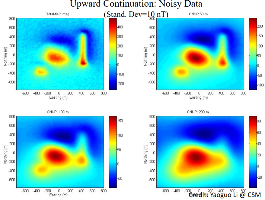
The same figure was reproduced using noisy data. Notice the significant difference between the accurate and noisy data at the lower elevations, and the reduction in noise as the responses are recorded at higher elevations of upward continuation.
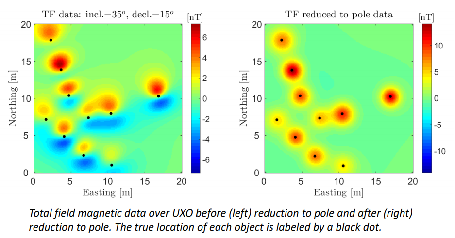
5.7. Reduction to pole
5.7.1. Fundamentals of reduction to pole
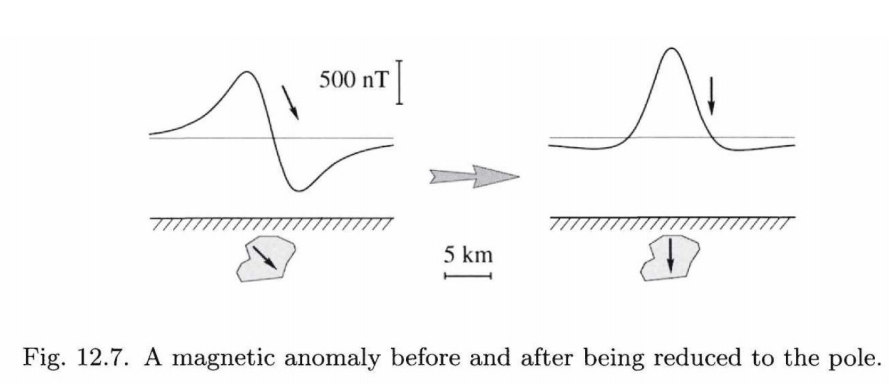
Reduction to Pole (RTP) is the process of adjusting recorded magnetic data so that it appears as if it was recorded if the Earth’s inducing magnetic field was vertical. The figure below shows this adjustment, and note the difference in terms of symmetry between the unadjusted and adjusted data. It is important to note that RTP is difficult to do at low magnetic inclinations (next to the equator).
The equation for RTP in the Fourier domain can be listed as the following:
![\[F[\Delta T_r] = F[\Delta T]F[\psi_r]\]](https://uhlibraries.pressbooks.pub/app/uploads/quicklatex/quicklatex.com-bd1511642ec765a2eed2891680ffcb87_l3.png "Rendered by QuickLaTeX.com")
![\[F[\psi] = \frac{1}{\Theta_m\Theta_f} = \frac{|k|^2}{(\vec{R}\cdot\hat{f})(\vec{R}\cdot\hat{m})}\]](https://uhlibraries.pressbooks.pub/app/uploads/quicklatex/quicklatex.com-b8466ca0ad11a12eae84bd73217521c2_l3.png "Rendered by QuickLaTeX.com")
![\[\vec{R} = (ik_x,ik_y,|k|)\]](https://uhlibraries.pressbooks.pub/app/uploads/quicklatex/quicklatex.com-3222d222d6a085fbc374de79db77e827_l3.png "Rendered by QuickLaTeX.com")
where  is the inducing field direction and
  is the magnetization direction
We can find the Fourier transform of RTP using the following three steps:
- Transform the observed data via FFT (Fast Fourier Transform)
- Multiply by

- Apply the inverse transform to obtain RTP
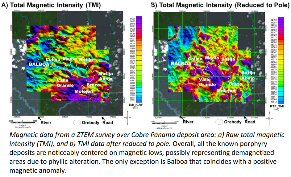
5.7.2. Examples of reduction to pole
5.8. Issues with fourier modelling
Throughout this chapter, we have gone through different methods in Fourier domain modelling using FFT (Fast Fourier Transform). However, FFT-based processing methods have two major prerequisites on data:
- The observation surface needs to be planar.
- Data needs to be interpolated to uniform grid.
These two prerequisites/assumptions is not made in practice because:
- Data are often acquired on undulating surface. For example, in an airborne survey with a helicopter, the flight height will be made constant to 50 m above the underlying terrain. However, the underlying terrain has a lot of hills and troughs. As such, the data measured by the helicopter is not from a planar surface because it follows the topography.
- Majority of data are acquired along flight lines or scattered stations. What this means is that the survey grid is not uniform in practice. For example, suppose an airborne survey using a helicopter. The helicopter will fly in one direction and obtain some measurements. After going through one survey line, it will move to the next survey line, which is around 100m away from the first survey line, and then it measures the data along that survey line. Now, the problem with this is that the data measured along the survey line (let’s say y direction, measurement every 5m) is much finer than data measured adjacent to the survey lines (let’s say x direction, measurement every 100m). Thus, you can have a grid of 5m x 100m. Clearly this grid is not uniform, and thus FFT will not work with this survey grid. One way to solve this problem is to use interpolation method but this has other problems as well
- The process of interpolation is a heavy processing step. Interpolation can be a dangerous process because it can create artifacts that does not exist in the data. Processed data maps would have many artifacts that would lead to misinterpretation.
In the next chapter, we will be going through a different method that does not produce artifacts in the data. This method is called the equivalent source method.
