Chapter 6: Interpretation methods

Jiajia Sun

6 Chapter 6: Interpretation methods

6.1. REVIEW OF GREEN’S FIRST & THIRD IDENTITY

Before going through equivalent source technique, it is best to review our understanding of Green’s theorem to understand the key concepts to this method.

6.1.1. Green’s first identity

Recall Green’s first identity, which is:

$\int \int \int_{Vol} (V \nabla^2 U + \nabla V \dot \nabla U) dv = \int \int_{Surf} V \frac{\partial U}{\partial \hat{n}} ds$

Where U, V are continuous functions with continuous first order partial derivative. U also has a second order derivative. An arbitrary vector $A = V\nabla U$ is also defined.

Now, assume that: U is harmonic and U=V, then:

$\int \int \int_{Vol} (\nabla U)^2 dv = \int \int_{Surf} U \frac{\partial U}{\partial \hat{n}} ds$

Let’s consider the above equation when U=0 on S. If that’s the case, then the right hand side of the equation vanishes.

Because the $(\nabla U)^2$ is always positive and continuous, then, that means:

$(\nabla U)^2 = 0$

This implies that U is constant. We have already assumed that U=0 on the surface. Because U is continuous, then that constant must be zero.

Therefore, if U is harmonic, U is continuously differentiable in R, and if U vanishes everywhere on the surface S, then U must also vanish everywhere within the volumes. Note that this only applies if the highlighted assumptions are true.

Now, consider two functions, $U_1$ and $U_2$ , be harmonic and have identical boundary conditions ( $U_1(S) = U_2(S)$ ). Thus, the function $U_1(S) - U_2(S)$ must be harmonic. Because $U_1 - U_2$ vanishes on S, then $U_1-U_2$ must vanish at every point. Therefore, $U_1$ is identical to $U_2$ . This implies that a function that is harmonic and continuously differentiable in R is uniquely determined by its value on surface S. Note that this only hold true if the highlighted assumptions are true.

What does it mean in potential field? Well, gravity and magnetic scalar potentials are harmonic and continously differentiable. Therefore, gravity and magnetic scalar potentials are uniquely determined by their values on S. As such: gravity and magnetic data are uniquely determined by their values on surface S.

Let’s use the following illustration to understand this concept.

Suppose that there are two density distributions as such:

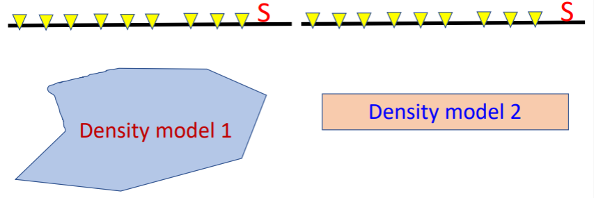
According to Green’s first identity, if the measurements on S are the same, then the gravity data from these two density models are the same. The two sources are called equivalent sources.

6.1.2. Green’s Third identity

Recall Green’s third identity. Considering the situation when V is harmonic:

$V(P) = \frac{1}{4\pi} \int\int_{Surf} (\frac{1}{r} \frac{\partial V}{\partial \hat{n}} - V\frac{\partial}{\partial \hat{n}}\frac{1}{r}) ds$

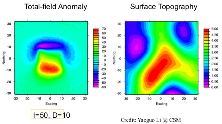
This implies that a harmonic function can be calculated at any point simply from its value and derivatives on the boundary (representation formula). Recall that this is used as a theoretical basis for upward continuation and equivalent source technique.

Because gravity/magnetic potential is harmonic, thus a potential field can be calculated at any point simply from the behavior of the field on the boundary. In other words, no knowledge about sources is required, except that none may be located within the region.

Unfortunately, Green’s third identity requires not only the values of V on the surface, but also the values of vertical derivative of ( $\frac{\partial V}{\partial \hat{n}}$ ). This is unlikely to be available in most practical applications. Fortunately, by some mathematical manipulations, we can eliminate the derivative from the equation.

Through some mathematical manipulations, Green’s third identity can be expressed as:

The above equation is called the upward-continuation integral. It shows how to calculate the value of a potential field at any point above a level, horizontal surface at $z_0$ from a complete knowledge of the field on the surface. The function also still implies that the potential field in R is determined by its values on S. Thus, upward continuation can be done in spatial domain using the above integral.

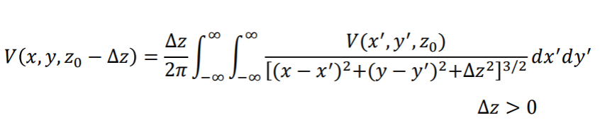
Let’s use the following example to understand this process.

Suppose that we do not know anything about density model 1. The anomaly from the source body is measured on S. Then, we can construct an equivalent source that reproduces the measurement on S using a known source body parameter, let’s say a rectangular density model pictured in Density model 2. The equivalent source (density model 2) will have zero resemblace to the true source body (density model 1). But this is still applicable in processing (to do UC, RTP,, component conversion, etc.), as long as it produces the same measurements on S. We can use equivalent source to calculate potential field values at any other locations in R.

Since we do not care what the equivalent source looks like as long as it produces the same measurements on S, we typically do not bother constructing a 3D equivalent source. Thus, we typically construct an equivalent source layer (i.e. a thin sheet of density) as the equivalent source.

There are several advantages to Equivalent source layer (ESL):

Free of the instabilities with RTP at low latitudes
Can do uneven-to-uneven surface continuation
Can use ESL to do RTP (Reduction-To-Pole), UC (Upward Continuation), component conversion, as we can work with ESL in Fourier domain.

The caveat is that to construct an equivalent source layer, we need to do an inversion.

6.2. EQUIVALENT SOURCE

Equivalent source is a very powerful image processing technique in processing and interpreting the potential field data. Almost all the data processing techniques we have talked about so far in Fourier domain can be accomplished by using equivalent source technique.

6.2.1. Inversion

After reviewing the Green’s first and third identity, we have built a solid theoretical understanding of the equivalent source technique now. However, in order to construct an equivalent source layer, we do need to do an inversion, which can be computationally expensive. Therefore, let us quickly go through the inversion firstly before we move on to the examples of applying the equivalent source technique.

Assuming that we have collected N number of discretized data samples on the surface of the Earth, which are denoted as a vector array as shown below.

$\vec{d}={{\left( {{d}_{1}},\cdots ,{{d}_{N}} \right)}^{T}}$

Then we need equivalent source that can be represented by point or piece-wise constant values (such as density or magnetization parameters) that can reproduce the collected data. The equivalent source can be mathematically denoted by a vector as follows:

$\vec{m}={{\left( {{m}_{1}},\cdots ,{{m}_{M}} \right)}^{T}}$

These two elements, the data measurements on the boundary and the equivalent source, are linked by a kernel matrix, $\mathbf{G}$ :

$\vec{d}=\mathbf{G}\vec{m}$

That is, given the measured data $\vec{d}$ , we want to construct $\vec{m}$ . Unfornately, we need to store the dense matrix $\mathbf{G}$ that requires large amount of memory and CPU time. For example, a 128 by 128 grid would require up to 1 Gb of memory to store this $\mathbf{G}$ matrix!

$\left[ \begin{matrix} {{g}_{11}} & {{g}_{12}} & \cdots & {{g}_{1M}} \\ {{g}_{21}} & {{g}_{22}} & {} & {} \\ \vdots & {} & \ddots & {} \\ {{g}_{N1}} & {} & {} & {{g}_{NM}} \\ \end{matrix} \right]\left[ \begin{matrix} {{m}_{1}} \\ {{m}_{2}} \\ \vdots \\ {{m}_{M}} \\ \end{matrix} \right]=\left[ \begin{matrix} {{d}_{1}} \\ {{d}_{2}} \\ \vdots \\ {{d}_{N}} \\ \end{matrix} \right]$

Moreover, the construction of $\vec{m}$ is often an ill-posed problem (we will discuss it in more details later). One way of mitigating this ill-posed problem is by the Tikhonov regularization method. That is, we formulate a cost function $\phi$ that consists of data misfit function ${{\phi }_{d}}$ , and the model objective function ${{\phi }_{m}}$ , these two terms are linked by a regularization parameter $\mu$ . Through minimizing the cost functional value $\phi$ , it is ensured that the reconstructed equivalent source parameters $\vec{m}$ can reproduce the measured data.

$\phi ={{\phi }_{d}}+\mu {{\phi }_{m}}$

6.2.2. Numerical Examples

6.2.2.1. Upward continuation

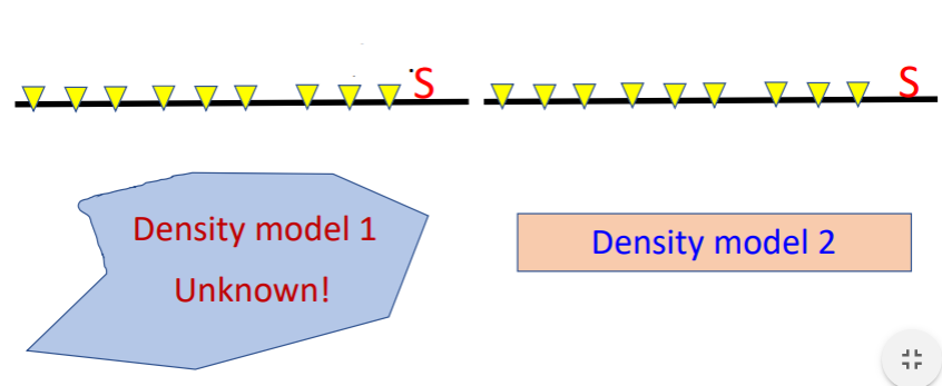
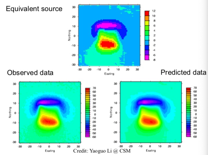
Here is a synthetic exampleof using equivalent source technique to do upward continuation.

The figure on the left is a synthetic total-field anomaly map that shows typical magnetic dipolar data pattern. This magnetic data is simulated by assuming the inclination equals 50 degrees, declination equals 10 degrees. The surface topography map displayed on the right can be interpreted as the data observation heights; that is, the observation data are not collected at an even surface.

Synthetic magnetic total-field anomaly data and its surface topography. Image courtesy of Yaoguo Li @ CSM

The reconstructed equivalent source layer (top plot) is displayed below. The reproduced data (bottom right plot) are simulated based on this equivalent source, and it is compared with the observed data map (bottom left plot) on the surface of the Earth.

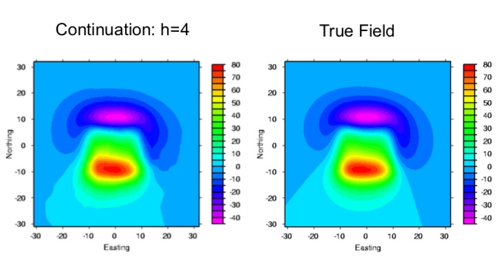
Constructed equivalent source layer and its corresponding data. Image courtesy of Yaoguo Li @ CSM

Since this recovered equivalent source can reproduce the measured data on the surface, therefore we will take this equivalent source layer to do upward continuation, as if it is the true source. The figure shown below is the upward continuation at 4 meters height (left plot), and it is compared with the true field measurement (right plot). These two plots look almost identical. Thus, this example proves that the equivalent source technique does work well.

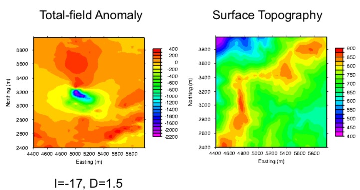
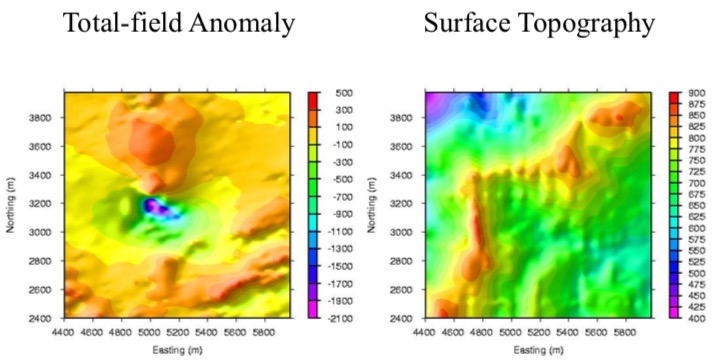
Upward continuation in comparison with the true field. Image courtesy of Yaoguo Li @ CSM

Here is another field example of using equivalent source technique to do upward continuation.

The magnetic map on the left figure below is collected from a low magnetic area with inclination of -17 degrees, declination of 1.5 degrees. The surface topography on the right map implies a very rough measurement height surface, with up to 500 meters variations. Since the data are not collected in a constant height, therefore we need to do upward continuation, and that requires an equivalent source layer.

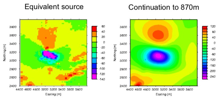
Field measured total-field anomaly data, and the surface topography. Image courtesy of Yaoguo Li @ CSM

After constructing and minimizing the objective functional value, given the measured total-field anomaly data, the reconstructed equivalent source layer is shown on the figure below (left plot). Then this equivalent source layer is used to do a forward modeling at the height of 870 meters above the Earth surface, the upward continued data simulated from this equivalent source is shown on right plot below.

Constructed equivalent source layer, and the upward-continued data based upon it. Image courtesy of Yaoguo Li @ CSM

6.2.2.2. Stable RTP

Equivalent source technique can also be used to do stable RTP even at low magnetic latitude.

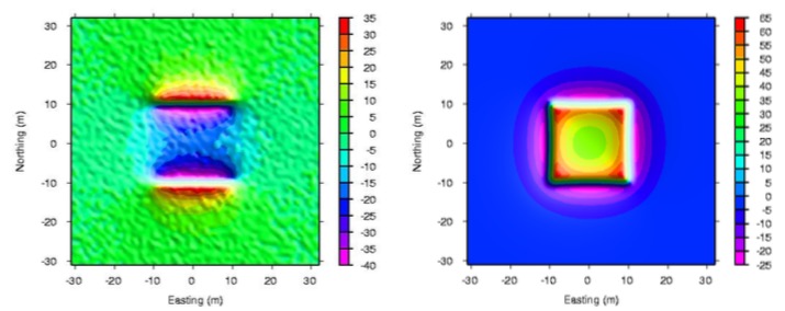
Here is a synthetic example. The left figure is the synthetically simulated TMI total-field anomaly data at a low magnetic latitude area; the data shows a typical positive-negative-positive pattern for magnetic data collected at low latitude region. The RTP in Fourier domain will be very challenging. Since this is a synthetic modeling, so we can use the true source to calculate the true RTP, which is displayed in the right plot below.

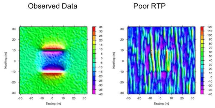
Synthetic TMI total-field anomaly data, and the true RTP. Image courtesy of Yaoguo Li @ CSM

If the noise is added into the clean total-field anomaly data (left plot below), then do the RTP by using the Fourier domain technique we talked about before, the resulted poor RTP figure shown on the right plot below has a lot of elongated strips artifacts along the direction of declination (0 degree in this example).

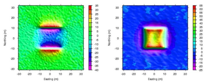
Observed data, and the computed poor RTP. Image courtesy of Yaoguo Li @ CSM

However, after using the magnetic data map (left plot below) to construct the equivalent source layer, then using the equivalent source layer to do the RTP (right plot below), the RTP quality is greatly improved.

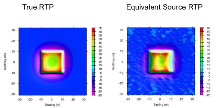
Observed data, with regularized RTP with positivity. Image courtesy of Yaoguo Li @ CSM

The equivalent source RTP is very similar with the true RTP, as shown in the comparison figure below, which is very interpretable.

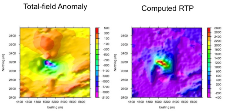
Comparison of the true RTP with the Equivalent source RTP. Image courtesy of Yaoguo Li @ CSM

Another is a field exampleof using equivalent source technique to compute RTP.

The measure total-field anomaly at a low magnetic latitude is shown on the left figure below, and its data collection surface topography (right plot) shows a 500 meters topography relief.

Measured data map, and the surface topography. Image courtesy of Yaoguo Li @ CSM

The computed RTP by using the equivalent source technique (right plot below) is very interpretable, since its peak anomaly lies on top of the anomaly body, and there are no elongated strips artifacts along the declination direction.

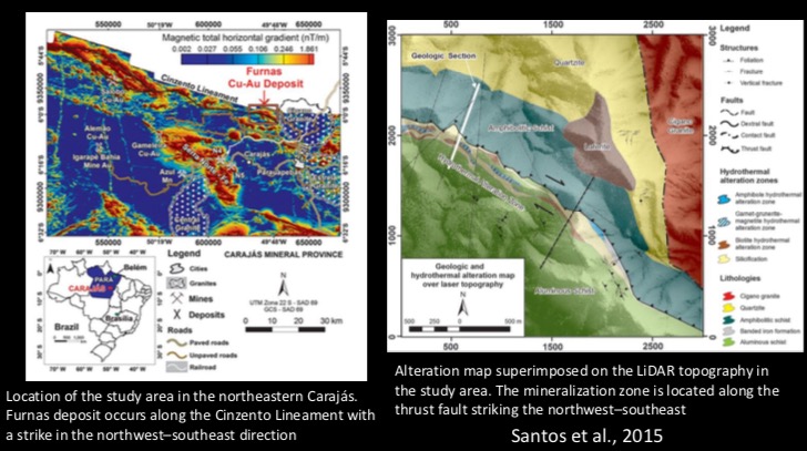
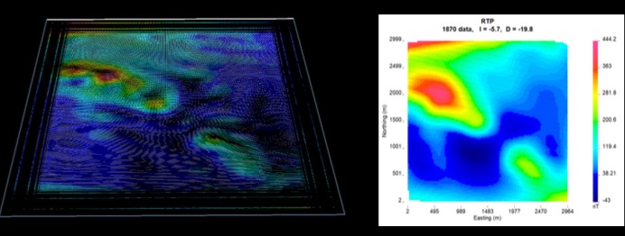
Measured data, and the computed Equivalent source RTP. Image courtesy of Yaoguo Li @ CSM

Here is another field example of using equivalent source technique to compute RTP at low latitude. The study area is in the northeastern Carajas, the interested mineralization zone is located along the major fault striking along the NW-SE direction. The simplified geologic unit map are shown in the figure below.

Study area location and the simplified geologic unit map. (Santos et al., 2015)

The collected magnetic data map was displayed in the figure below. Although it shows a typical positive-negative magnetic data pattern, it is very challenging to deal with due to various conditions. Firstly, the data are from very low latitude of -5.7 degrees; Secondly, the data has strong remanence; moreover, it is self-demag and affected by anisotropy.

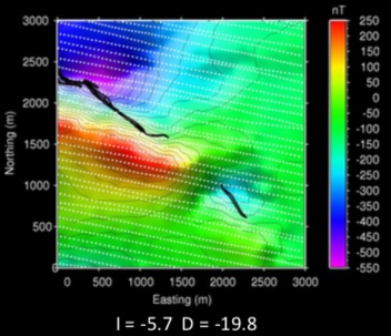
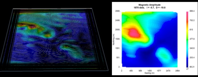
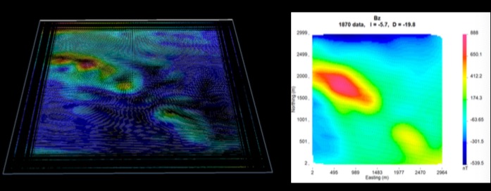
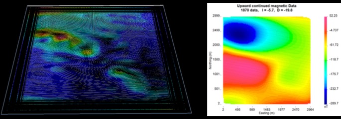
The measured magnetic data. (Leao-Santos et al., 2015)

However, after applying the equivalent source technique, the data is much easier to work with. The equivalent source layer was constructed, and then it can be used to compute the RTP, the magnetic amplitude, the magnetic component Bx, By, Bz, or the upward continuation, since this equivalent source layer is able to reproduce the observed data on the surface of the Earth.

Constructed equivalent source layer, and the RTP.

Constructed equivalent source layer, and the magnetic amplitude.

Constructed equivalent source layer, and the Bz component.

Constructed equivalent source layer, and the upward continuation at 800 m.

6.3. Depth estimates

6.3.1. Half width method

Shown in the figure below, assuming there is a small ore body in the subsurface. It is the spherical shape with a radius of 10 m, located at a depth of 25m and the density contrast is 0.5 gm/cc. We are going to look at the gravity of the uniform sphere at different depth.

Gravity due to a uniform sphere where depth=25 m.

Gravity due to a uniform sphere where depth=50 m.

Gravity due to a uniform sphere where depth=100 m.

Gravity due to a uniform sphere where depth=200 m.

Gravity due to a uniform sphere where depth=400 m.

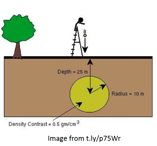
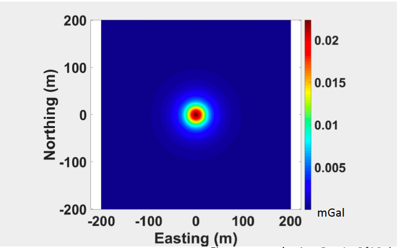
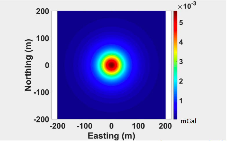
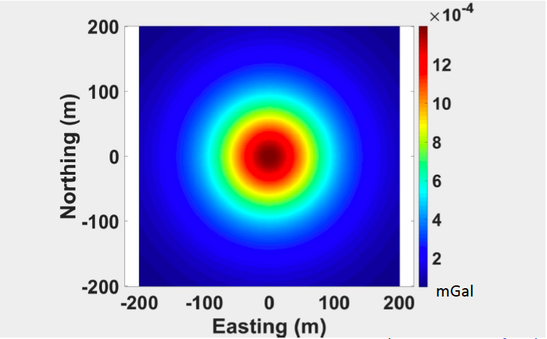
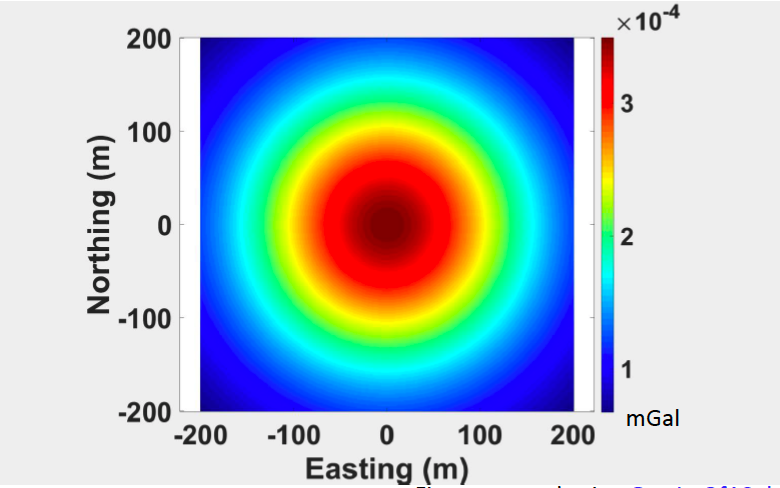
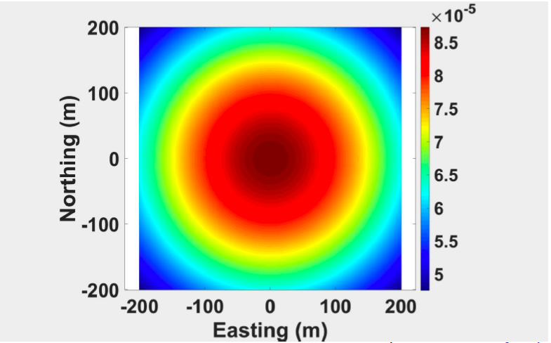
Everything is same in the above 5 figures, the radius is same, the geometry of anomaly is same. The only thing different is the depth changing from the shallower to deeper.

We can observe from the above figures that the maximum gravity measure decreases as depth increases. Besides, the width of the central peak region increases.

Let’s look at a profile of gravity at depth = 25 m (seeing figure below), where the red line is profile.

We plot the gravity of this profile shown in below:

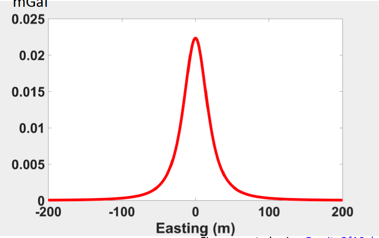
A profile (Northing = 0 m) of the gravity measures, where anomaly body located at depth = 25 m.

The observations from the figure above, the location at 0 corresponds to the location of source body and the peak located directly above the center of the anomaly body. The same things when we change the depth while keeping the same profile position (figures below).

A profile (Northing = 0 m) of the gravity measures, where anomaly body located at depth = 50 m.

A profile (Northing = 0 m) of the gravity measures, where anomaly body located at depth = 100 m.

A profile (Northing = 0 m) of the gravity measures, where anomaly body located at depth = 200 m.

A profile (Northing = 0 m) of the gravity measures, where anomaly body located at depth = 400 m.

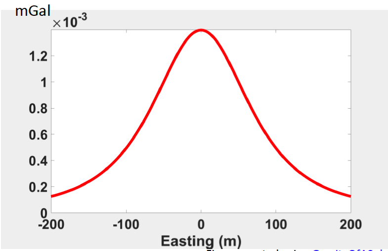
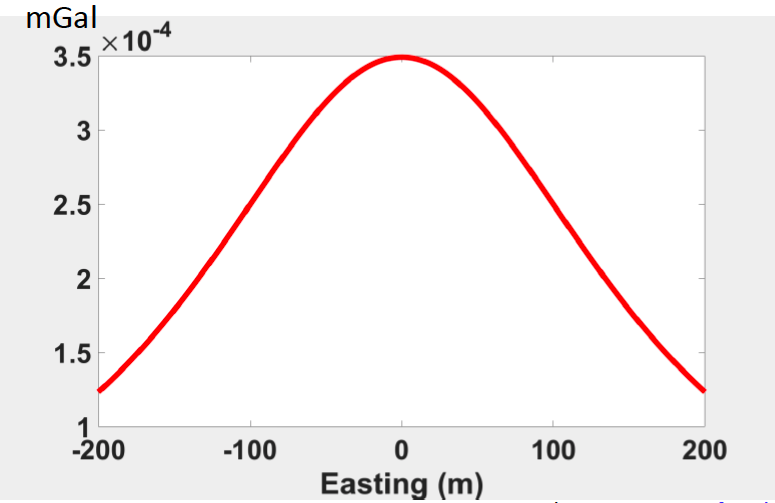
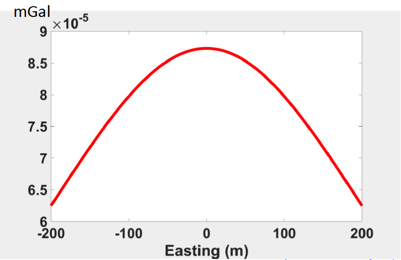
Here, we observe two thing from the figures above: Firstly, the maximum value (peak) decreases as depth increases. Secondly, width of the central peak region increases. These two trends are same with 2D maps of gravity measures.

Question

Can we use width to estimate depth???

Yes, we can!

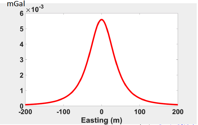
We noticed there are some correlation between width of the peak and depth. The width seems to be depended on the depth. So logically speaking, we can use the width to estimate the depth of source body. Let’s take a careful look at the profile at depth = 50 m.

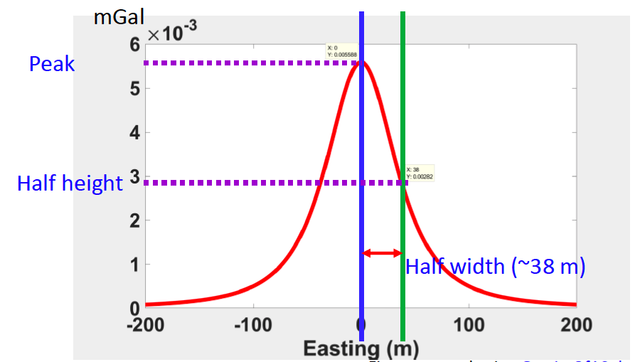
Observation from the figure above, the peak value is 0.0055. The blue line is location of peak. The green line is the position of half of peak value, and at this point the value is 0.00282. The distance between blue line and green line is half width. In this particular case, the half width is 38 m.

There is a rule of thumb that we can use to estimate depth for spheres:

$depth = 1.3 * half-width$

In the equation, the depth is really the vertical distance between your observation and the center of the sphere. Thus, in our particular example, the depth = 1.3 * 38 = 49.4 m, which is really close to the true depth 50 m.

The half-width rule of thumb estimates depth for cylinders:

$depth = 1.0 * half-width$

The half-width rule of thumb is a practical rule, but there is a limitation that is we have to assume the shape of source body. If the source body is assumed to be sphere, we need to use 1.3 * half-width. In comparison, if it is a cylinder, we need to use 1.0 * half-width.

6.3.2. Rules of thumb for maximum depth

Firstly, we make clear of a term: non-uniqueness. Many geologically reasonable density or magnetization solutions may perfectly satisfy the observed anomaly, which means the many potential correct models can fit our observed gravity or magnetic data equally well. For example, gravity due to s sphere is the same as a point mass. Because of non-uniqueness, actually we can create multiple source bodies and each of created source body can fit our observed data. However, some parameters about the source bodies can be uniquely determined from the observed anomalies, without assumptions about the source distribution (Blakely, 1996, p239), eg., maximum depth.

We are going to talk how to estimate maximum depth. The first question is what is maximum depth.

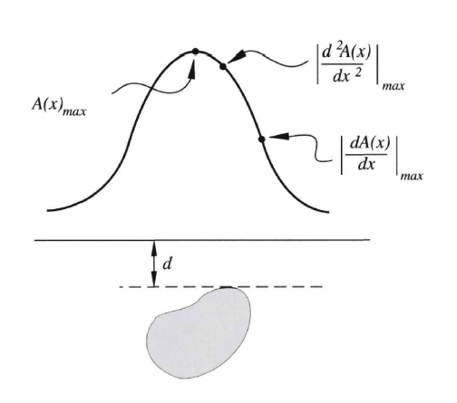
Maximum depth to causative sources based on first, second, and third derivatives fo their anomalies. Profile A(x) represents either a magnetic or gravity anomaly. (Blakely, 1996, p240)

The black curve is gravity or magnetic measures. The depth to a plane (the dash line shown above) below which the entire source distribution lies, which is represented by ‘d’ in the figure above. The maximum depth ‘d’ can be determined based on first, second or third derivatives of gravity or magnetic anomalies along profiles. We can use the information from derivative to help us estimate the depth.

We can estimate maximum depth for 3D gravity anomalies using the following equations (Blakely, 1996, p240):

$d\leqslant5.40\;\frac{\gamma\rho_{max}}{{\left|A''\right|}_{max}}$

$d^2\leqslant6.26\;\frac{\gamma\rho_{max}}{{\left|A'''\right|}_{max}}$

where, the density of both signs that means the gravity anomalies could be both positive and negative. $\gamma$ is gravitational constant. $\rho_{max}$ is maximum density value. ${\left|A''\right|}_{max}$ is maximum value of the second order derivative. ${\left|A'''\right|}_{max}$ is maximum value of the third order derivative.

For both above equations, the upper limitation of maximum depth is right hand side. If we wanna use it to estimate maximum depth, we have to roughly estimate the maximum density value $\rho_{max}$ . For example, we can estimate the maximum density value through measures of crops, borehole gravity measurements or our basic understanding of rocks. Here is a specific example to show what’s the meaning of these two equations. If we measures the maximum depth is 400 meters, which means the depth of source body cannot be deeper than 400 m.

If the density entirely positive or entirely negative rather density of both signs, there are many other extra rules we can use to estimate the maximum depth.

$d\leqslant1.5\;\frac{A}{{\left|A'\right|}}$

where the rule is for all x.

$d^2\leqslant-3\;\frac{A}{A''}$

where the rule is for all x and $A''$ is negative.

$d\leqslant0.86\;\frac{A_{max}}{{\left|A'\right|}_{max}}$

$d\leqslant2.70\;\frac{\gamma\rho_{max}}{{\left|A''\right|}_{max}}$

$d^2\leqslant3.13\;\frac{\gamma\rho_{max}}{{\left|A'''\right|}_{max}}$

All these five rules above can help us estimate the maximum depth. We are going to talk about one rule specifically.

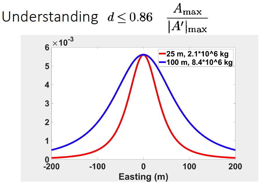
In the rule $d<0.86\;\frac{A_{max}}{{\left|A'\right|}_{max}}$ , we don’t need estimate maximum density value, which is more convenient to use. In the figure, we have two gravity profiles. These two profile have same maximum value because of peak is overlap with each other. The red curve decay faster than blue curve that means the first order derivative of red curve is larger than blue curve. Therefore, the maximum depth of blue curve is deeper than red curve, because the denominator of red curve is larger than blue cure. Another way to understand this is based on the first method we talked before, the half-width of the blue curve is larger than red, so the depth of blue curve is deeper than red curve.

The rules to estimate the maximum depth for 2D gravity anomalies are shown below:

$d\leqslant\frac{A}{{\left|A'\right|}}$

where the rule is for all x.

$d^2\leqslant-2\;\frac{A}{A''}$

where the rule is for all x and $A''$ is negative.

$d\leqslant0.65\;\frac{A_{max}}{{\left|A'\right|}_{max}}$

$d\leqslant\triangle\omega$

where the rule is for symmetric anomaly.

The maximum depth estimation for 3D magnetic anomalies are following:

No restrictions on magnetization:

$d\leqslant6.28\left(4\widehat r_x^2+3\widehat r_y^2+3\widehat r_z^2\right)^{0.5}\;\frac{M_{max}}{{\left|A'\right|}_{max}}$

$d^2\leqslant9.73\left(3\widehat r_x^2+2\widehat r_y^2+2\widehat r_z^2\right)^{0.5}\;\frac{M_{max}}{{\left|A''\right|}_{max}}$

Magnetization everywhere parallel and same sense:

$d\leqslant3.14\left(4\widehat r_x^2+3\widehat r_y^2+3\widehat r_z^2\right)^{0.5}\;\frac{M_{max}}{{\left|A'\right|}_{max}}$

$d^2\leqslant4.87\left(3\widehat r_x^2+2\widehat r_y^2+2\widehat r_z^2\right)^{0.5}\;\frac{M_{max}}{{\left|A''\right|}_{max}}$

Vertical $\widehat r$ and vertical $\mathbf{M}$ :

$d\leqslant5.18\;\frac{M_{max}}{{\left|A'\right|}_{max}}$

$d^2\leqslant6.28\;\frac{M_{max}}{{\left|A''\right|}_{max}}$

Vertical $\widehat r$ and vertical $\mathbf{M}$ ; $\mathbf{M}$ everywhere of same sense:

$d\leqslant2.59\;\frac{M_{max}}{{\left|A'\right|}_{max}}$

$d^2\leqslant3.14\;\frac{M_{max}}{{\left|A''\right|}_{max}}$

where $\mathbf{M}_{max}$ is maximum value of magnetization. $\widehat r=({\widehat r}_x,{\widehat r}_y,{\widehat r}_z)$ is direction in which magnetic field is measured.

The maximum depth estimation for =2D magnetic anomalies are following:

No restrictions on magnetization:

$d\leqslant8\left(\widehat r_x^2+\widehat r_z^2\right)^{0.5}\;\frac{M_{max}}{{\left|A'\right|}_{max}}$

$d^2\leqslant9.42\left(\widehat r_x^2+\widehat r_z^2\right)^{0.5}\;\frac{M_{max}}{{\left|A''\right|}_{max}}$

$\mathbf{M}$ everywhere parallel and same sense:

$d\leqslant4\left(\widehat r_x^2+\widehat r_z^2\right)^{0.5}\;\frac{M_{max}}{{\left|A'\right|}_{max}}$

$d^2\leqslant4.71\left(\widehat r_x^2+\widehat r_z^2\right)^{0.5}\;\frac{M_{max}}{{\left|A''\right|}_{max}}$

6.3.3. Euler deconvolution

The previous methods of depth estimation that we covered are best suited for anomalies caused by single and isolated bodies. However, there is another class of techniques that consider magnetic or gravity anomalies caused by multiple and relatively simple sources. One of these methods is Euler Deconvolution. In order to understand Euler Deconvolution, we need to recall Harmonic functions.

6.3.3.1 Harmonic Functions

$\nabla^2V = 0$

If the Laplacian of a vector $V$ is equal to zero, then $V$ is a harmonic function. Additionally, any spacial derivative of a harmonic function is also harmonic. The spatial derivatives and Laplacian operator are also commutative. E.g., $\nabla^2(\frac{\partial}{\partial x}V) = \frac{\partial}{\partial x}(\nabla^2V)$ . This means that we can generate a host of harmonic functions from a given harmonic function. For example, if we consider the vector (\frac{1}{r}), we know that it is harmonic as $\nabla^2\frac{1}{r} = 0$ . It therefore follows that $\frac{\partial}{\partial z}\frac{1}{r}$ , $\nabla \frac{1}{r}$ , and $m \cdot \nabla \frac{1}{r}$ are all harmonic. The last harmonic function listed is important to remember, as it describes the magnetic potential of a dipole. Here, we can note that the scalar magnetic potential is harmonic, which also means that any component of the Earth’s magnetic field is also harmonic. This is because any component of the magnetic field is simply a spacial derivative of the potential.

6.3.3.2 Homogeneous Functions

A function $V$ is homogeneous of degree $n$ if it satisfies Euler’s equation:

$x \frac{\partial V}{\partial x} + y \frac{\partial V}{\partial y} + z \frac{\partial V}{\partial z} = nV$

In a simple example, if $V=xyz$ , we can state that $V$ is homogeneous of degree 3. Similarly, $V=xy$ is homogeneous of degree 2 and $V=x$ of degree 1. In a more complex example, we can analyze $V=log\frac{r+z}{r-z}$ which is homogeneous of degree 0. Similarly, $V=\frac{1}{r}$ is homogeneous of degree -1 and V= $\frac{z}{r^3}$ of degree -2. For any vector $V$ , if it is homogeneous then any derivative of $V$ is also homogeneous. As we established previously, $\frac{1}{r}$ is homogeneous and therefore the potential of a magnetic dipole is too.

If a homogeneous function is also harmonic, it can be represented in spherical coordinates as a sum of spherical surface harmonics.

6.3.3.3 Euler’s Equation

We can express Euler’s equation using the following general form:

$r \cdot \nabla f = -nf$

In this form, it is easy to show that $f = \frac{1}{r}$ satisfies Euler’s equation with $n=1$ . Therefore, the potential of a point mass must also be homogeneous with $n=1$ . Next, we will take a look at the total-field anomaly of a dipole:

$\Delta T = \frac{mu_0}{4\pi} \hat{b} \cdot \nabla(m \cdot \frac{1}{r})$

This equation satisfies Euler’s equation with $n=3$ .

Next, let us consider a magnetic survey. We will set $\Delta T_i$ as the ith measurement at location (x,y,z). Additionally, we will assume the center of the source body is at location $(x_0, y_0, z_0)$ . We can represent this survey according to Euler’s equation:

$[\frac{\partial}{\partial x} \Delta T_i \quad \frac{\partial}{\partial y} \Delta T_i \quad \frac{\partial}{\partial z} \Delta T_i] \begin{bmatrix} x - x_0\\ y - y_0\\ z - z_0\\ \end{bmatrix} = n \Delta T_i$

Similarly, other measurements at other locations can be represented by expanding the previous equation:

$\begin{bmatrix} \frac{\partial}{\partial x} \Delta T_1 & \frac{\partial}{\partial y} \Delta T_1 & \frac{\partial}{\partial z} \Delta T_1 \\ \frac{\partial}{\partial x} \Delta T_2 & \frac{\partial}{\partial y} \Delta T_2 & \frac{\partial}{\partial z} \Delta T_2 \\ \vdots & \vdots & \vdots \\ \end{bmatrix} \begin{bmatrix} x - x_0\\ y - y_0\\ z - z_0\\ \end{bmatrix} = \begin{bmatrix} n \Delta T_1 \\ n \Delta T_2 \\ \vdots \\ \end{bmatrix}$

We can solve this equation using a least-squares method for $(x_0, y_0, z_0)$ if we assume a value of $n$ .

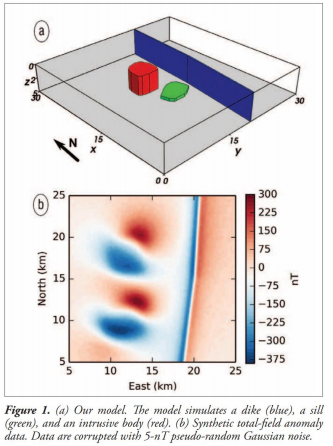
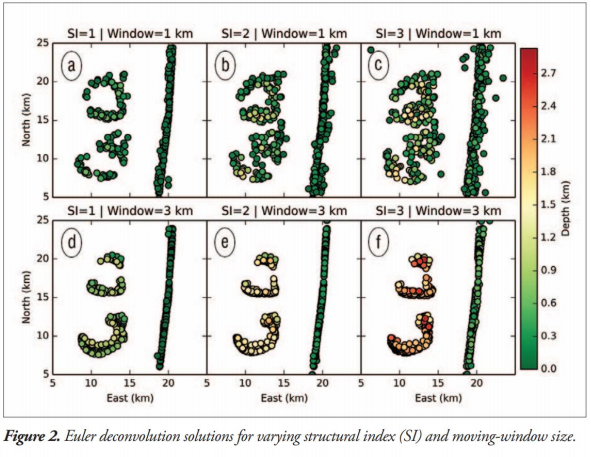
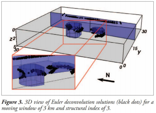
6.3.3.4 Example of Euler’s Deconvolution

The example used below comes from a Geophysics Tutorial by Leonardo Uieda, Vanderlei C. Oliveira Jr, and Valéria C. F. Barbosa.
Uieda, L., V. C. Oliveira Jr, and V. C. F. Barbosa (2014), Geophysical tutorial: Euler deconvolution of potential-field data, The Leading Edge, 33(4), 448-450, doi:10.1190/tle33040448.1

6.3.4. Spectral Depth Estimation

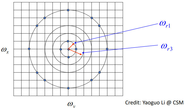
Spectral depth estimation is done by calculating the radially averaged power spectrum of potential field data using the Fourier Transform. It is found by taking the average over points on concentric circles followed by smoothing along radial wave numbers. An example is shown in the figure below.

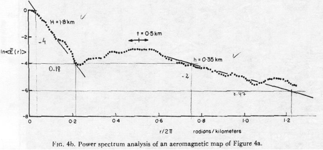
There a couple of important properties related to the radially averaged power spectrum for single source bodies that we will discuss. In regards to the decay of the power spectra of gravity and magnetic data, this decay depends primarily on the source depth. Deeper source depths result in faster decay of the power spectra, also leading to narrower recorded bandwidth. A semi-log plot can be used to plot the radially averaged power spectra, as parts of the spectra will appear as straight line segments. The slope of these line segments is proportional to the source depth, and can be described using this equation:

$ln[p(w_r)] \propto 2lnw_r - 2hw_r$

Note that in the intermediate wavenumber band, the slope is proportional to twice the source depth.

We will briefly discuss a paper by Spector and Grant (1970) on the Ensemble Average and power spectra. In this paper, an ensemble of rectangular prisms were used to represent parameters that were randomly distributed, uncorrelated, and had uniform probability. They used this to examine the expected power spectra of a magnetic field, and reached some surprising conclusions.

$p_B(w_r)\propto e^{-2\bar{h}w_r}$

if $\Delta h << \bar{h}$

In this case, $\bar{h}$ is the average central depth of the ensemble and $2\Deltah$ is the depth interval within which $h$ is uniformly distributed. The authors concluded that the power spectrum of the ensemble behaves the same as an “average” member from within the ensemble.

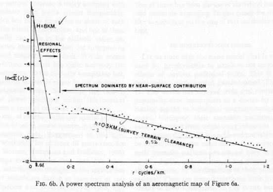
Next, we will take a look at field data collected from Kirtland.

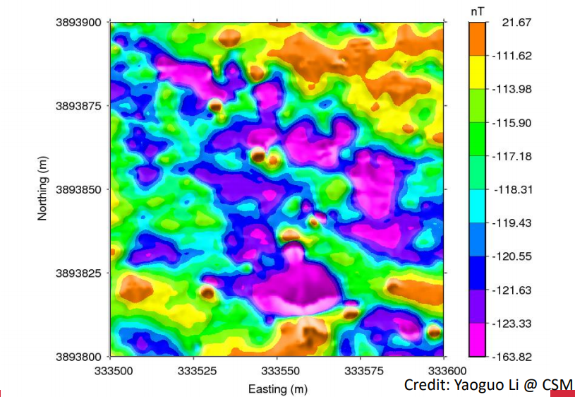
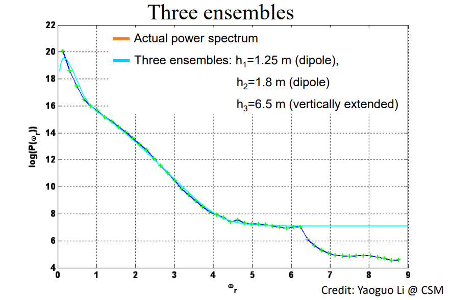
Airborne magnetic data collected over Kirtland

The radially averaged power spectrum of the Kirtland data, with the power spectra of three rectangular ensembles compared to the actual power spectrum

Note that with the radially averaged power spectrum of the Kirtland data, the majority of the rectangular ensembles match the actual power spectrum almost perfectly, confirming the results of the Spector and Grant paper.

License

Icon for the Creative Commons Attribution-NonCommercial 4.0 International License