3.1 Gravity Instrument

By now, we have accumulated the basic understandings of the gravity theories, now let us put things in perspective. Assume earth’s gravity is approximately 9.8 , that is, 980 Gal. The anomalies that we typically see in geoscience applications are typically less than 100 mgal, which is less than 0.01% (one part in 10⁴) of the Earth’s average gravity field. Therefore, if our interested anomaly is 10 mgal, we are then looking for a tiny signal that is one part in 10⁵! If our signal is 10 , then the tiny signal we will be looking for is only about one part in 10⁸!!

3.1.1 How to measure gravity?

So how to measure gravity to catch the tiny signals caused by our interested anomaly targets? There are generally three kinds of measurements to get either the absolute gravity or the relative gravity data. These methods are

• Falling body measurements
  • Which is simply to drop an object, and measure the distance and time, then calculate the (absolute) gravitational acceleration.
• Pendulum measurements
  • Which is to measure the period of oscillation of a pendulum.
• Mass on spring measurements
  • Which is to suspend a mass on a spring and measure the amount of the stretch of the spring under the force of gravity.

Let us discuss these methods and the gravity instruments designed based on them in more detail.

3.1.1.1 Falling body measurements

The basic principle applied in the falling body measurements is the free fall, which is any motion of a body where gravity is the only force acting upon it, as illustrated in the cartoon images shown below.

From what we have learned from Physics lectures, we have known that the final velocity at a later time can be calculated from the velocity as an earlier time, along with gravity acceleration and the traveling time, which is

Where g is the time rate of change of speed (i.e., acceleration). Therefore, we can calculate the gravity acceleration through the time difference and the speeds.
However, in the actual practice, it is very hard to measure velocity accurately. But we can measure the traveled distance more precisely and easily. So, if we assume the initial velocity is zero, then the distance traveled can be expressed as follows:

Thus, the absolute gravity g can be then calculated from the measurement of distance and time.

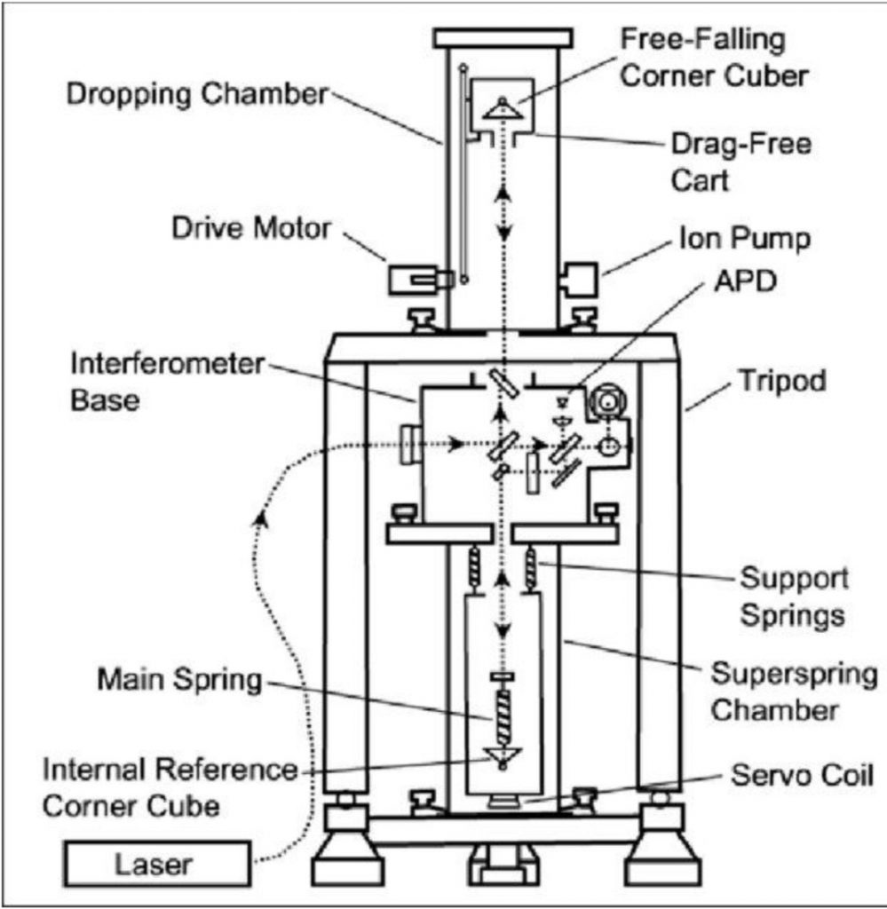
One of the example instruments designed based on the free fall principle is the Absolute gravimeter FG-5 by the Micro g LaCoste company. Its schematic diagram is shown below, which consists of three sections. The upper section is a vacuum dropping chamber, where a mass drops at roughly 100 cycles/minute. The middle section contains an interferometer to measure the position of the falling mass. The lower section has spring systems that prevent the free-fall system from being affected by Earth vibrations, therefore it functions as a cushion center to stabilize the whole gravimeter system. The reported absolute accuracy of this instrument is , with the measurement precision of .

Measuring absolute gravity is very very challenging! To measure gravity down to 1 part in 40 million (i.e., 25 ) using an instrument of reasonable size (e.g., one that allows an object to drop 1 meter), we need to be able to measure changes in distance down to 1 part in 10 millions and changes in time down to 1 part in 100 millions!
For example, let us assume a small ore body (indicated as the yellow circle in the graph below), in a spherical shape with a radius of 10 meters, centered at the depth of 25 meters below the ground surface. The density contrast of it with its surrounding sediments is 0.5 g/cc. The measured gravity data along a line profile above the ore body will be symmetrical about the center of the sphere. The maximum value is quite small, with about 25 , and the gravity data approach 0 at a further distance away from the anomaly center (here beyond 60 m).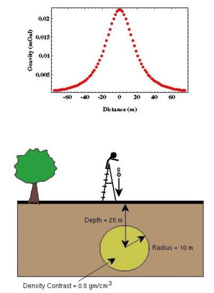

3.1.1.2 Pendulum measurements

Another method to measure absolute gravity is through the pendulum measurements. The principle is that we can build a simple pendulum by hanging a mass from a rod and displacing it from the vertical, like the setting shown in the picture on the left.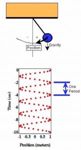 The mass will begin to oscillate back and forth. The gravity will determine the period of its oscillation; if the gravity is small, there is less force pulling the mass downward, therefore, the pendulum will move slowly toward the vertical, and resulting a longer oscillation period. The math expression for gravity and the period is as follows:

The equation is assumed to be true when there is no friction involved in the motion. is a constant controlled by the physical characteristics of the pendulum such as its length and the distribution of the mass. This equation will give us absolute gravity measurements.

Historically, pendulum measurements were used extensively to measure the gravitational acceleration around the globe. To minimize the error, many periods of oscillations were observed then the average of them would be used.

Unfortunately, the measurement of constant is not accurate enough to allow us to make gravity measurements down to 1 part in 40 million precision. Often the accuracy is limited to roughly 0.1 (Hinze et al., 2017, p103).

Although we cannot measure accurately, if we use the same pendulum system, the value is constant, then by using the same pendulum to measure the periods of oscillation at two different locations, we can estimate the change in gravitational acceleration at these two locations, without knowing . This method gives us the relative gravity measurement.

For example, the figure below shows the comparison of absolute and relative gravity measurements for the same study region. Notice that, the shapes of the two gravity profiles are the same, the only difference is a constant offset; the anomaly absolute density value was replaced with the density contrast value in the relative gravity measurement setting. Relative gravity measurements contain all the information we need to identify the location and shape of the ore body since what matters is the change in gravity, not the absolute gravity values. Thus the relevant parameter is the density contrast, not the density itself.

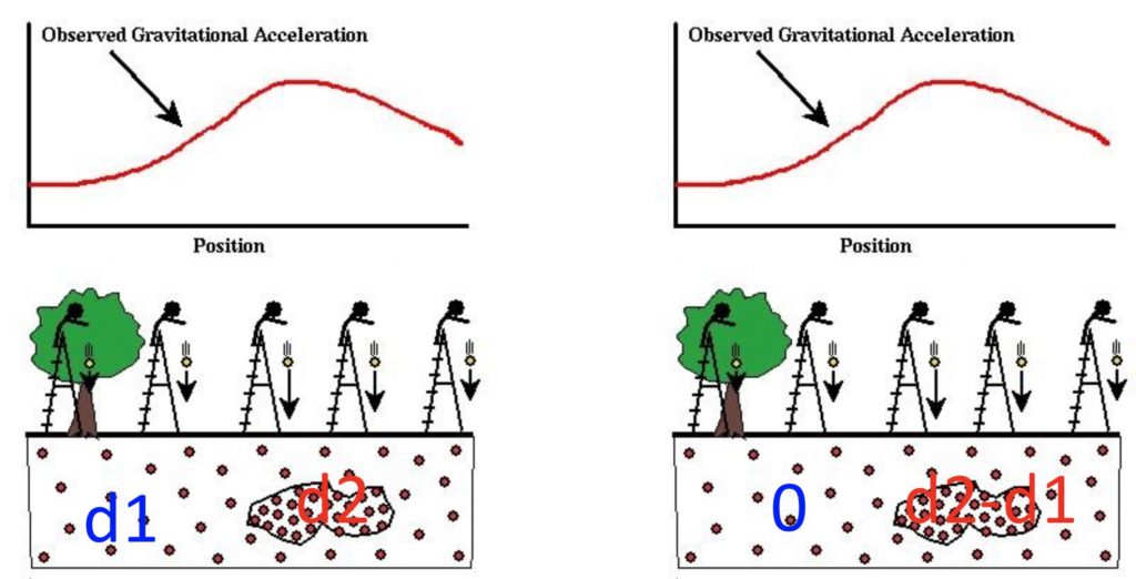
3.1.1.3 Mass on spring measurements

Gravity can also be measured with a mass-spring system. As shown in the figure on the left,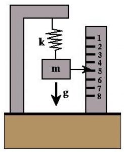 the principle is that, if a mass is hung on a spring, the spring will be stretched because of the gravity force acting upon the mass. The stretch is proportional to gravity, mathematically expressed as follows:

Where is the stiffness of the spring, the larger the is, the stiffer the spring is, and the less the spring would be stretched.

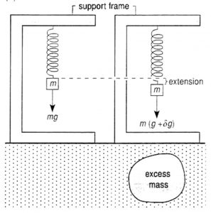
Again, we cannot measure value accurately enough to make sure the measured gravity precision down to 1 part in 40 million. However, the extension is proportional to the change in gravity caused by the change in density. Therefore, we can measure relative gravity (i.e., gravity change) by measuring the extension, as illustrated in the experiment set in the graph below.

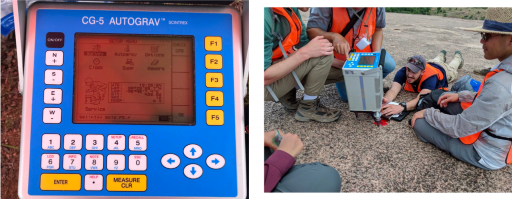
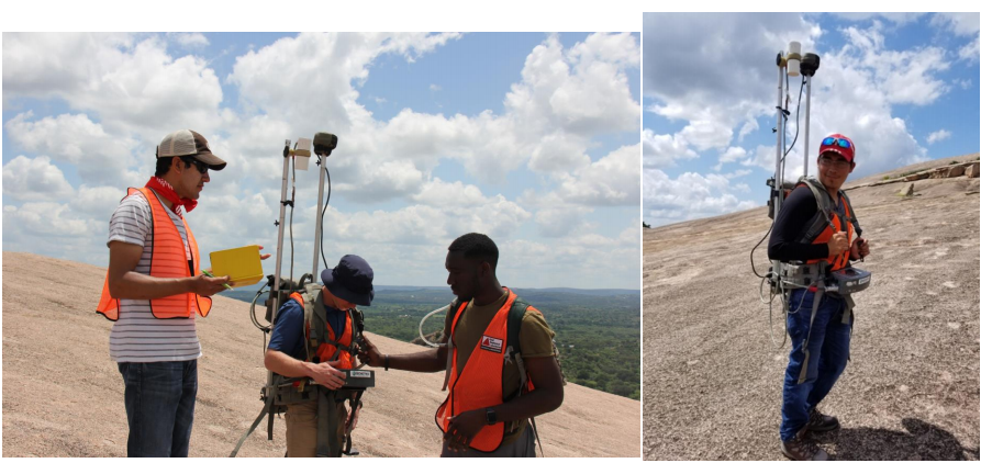
One of the gravimeter examples using this mass-spring measurement system is the CG5 gravimeter, used often in the UH Geophysical Field Camp, as shown in the picture below.

3.1.1.4 Absolute vs. Relative gravimeter

In terms of measurement accuracy, relative gravimeters usually have an accuracy of > , while absolute gravimeters can have accuracies on the order of 1 . For the instrument itself, absolute gravimeters are usually larger and heavier than relative gravimeters. Therefore, using absolute gravimeters will take longer measurement time, and more expensive.
However, absolute gravity measurements are more accurate, and the measured data are free from instrument drift corrections. Therefore, their measured data can be used to establish reference points to tie together individual surveys, to both national and international datums, and can be used to establish gravity benchmarks. They are also useful for studies involving high-precision time variations in gravity, for instance, it is possible to observe a 3 mm crustal uplift by monitoring the change in gravity at a single station.

3.1.1.5 Satellite gravimeter

Gravity measurements can also be taken by designed satellites. One of the well-known examples is the Gravity Recovery and Climate Experiment (GRACE) mission, which was a joint mission of NASA and the German Aerospace Center launched in March 2002 and ended in October 2017. This mission was operated by two twin satellites which could take detailed measurements of Earth’s gravity field and its changes over time. Their measured data were used for studying Earth’s ocean, geology, climate, and hydrology, etc.

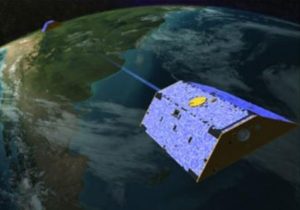
Their working principle is that the two identical satellites, each about the size of a car, were separate 220 km (137 miles) apart, one following the other around the Earth. A microwave ranging system in the satellites could measure the distance between them to within a micrometer (0.001 mm), which is smaller than a red blood cell. By measuring the tiny changes in distance between them, we were able to measure the subtle changes in gravity, since their distance changes are caused by each of them speeds up and slows down in response to the gravitational force. A successful case study done by using the GRACE data is the measurement of the water storage in Amazon.

3.2 Gravity data processing:

3.2.1 Contributions to gravity

The observed gravity measurement that we get from gravity instruments (i.e. CG-5) are due to many factors. The observed gravity measurements are a summation of the following contributors:

1. Attraction of the reference ellipsoid: Accounts for 99% of your gravity measurements. It is the gravity due to the earth, which has an ellipsoidal shape. Recall that the gravitational attraction in the equator is smaller than the poles because due to the ellipsoidal shape of the earth.
2. Effect of earth’s rotation: The gravity due to the earth spinning on its axis. Recall that the centrifugal force is stronger in the equator, which makes the gravitational attraction in the equator to be smaller than in the poles.
3. Instrument drift: The gravity measurements from relative gravity instruments (such as CG-5) is not consistent with time due to the spring-mass system inside the instrument. The change of k (spring constant) in the spring affects the gravity readings from the instrument (not a real change in the gravity field)
4. Effect of elevation: The gravitational attraction in different observation elevation are different simply because the observation locations will have different distances towards the center of the earth
5. Effect of mass above sea level: The earth is not a simple flat plain, it also has mountains and other features above the sea level that will also have its own gravitational attraction to the gravity instrument and account for the observed gravity measurement
6. Effect of topography: The earth’s surface is subject to different topography (i.e. mountains, troughs, valleys, etc.) and therefore our measurements are also subject to this effect as well (similar reasoning to mass above sea level).
7. Effect of compensating masses at depth: The earth’s crust has different density and thickness throughout the earth. This also accounts for the gravity measurements.
8. Effect of moving platform: If we measure gravity in a moving platform, such as airplanes, helicopter, boat, etc, then even the movements and rumblings that is caused by the movement can contribute to the gravity measurements.
9. Effect of local geology of interest: Gravity due to density variations in the crust. This is caused by the density contrasts in the subsurface, which gives clues on what geological features exist in the subsurface. This effect is what we want to isolate and use for interpreting geology.

In geophysics, the gravity that we are interested in is the effect of local geology of interest, which will give us information on the density contrast in the subsurface, and interpret the geology based on the measurements. However, in order to get this information, that means we need to correctly find the gravity contribution from the 8 other effects, and subtract the observed gravity with them. Putting it in a more mathematical perspective:

The process of subtracting these contributions from the observed gravity is called gravity data correction. This involves modelling/finding each of the gravity contributions so that we can subtract them from the observed gravity to find the gravity from the geology of interest. There are different types of corrections that account for each of these effects, which we will learn in the next section.

• Theoretical Gravity: Gravity attraction from the reference ellipsoid and effect of the earth’s rotation. Generally, this correction has something to do with the latitude position of the measurements. This has been discussed in the previous section, as the theoretical gravity can be expressed as:

Where ge is the gravitational attraction in the equator, is the latitude.

• Temporal Correction: Like the name suggested, this correction has something to do with changes in gravity measurements with time. This includes the correction for effects of tides and instrument drift. 

• Free-air Correction: This correction accounts for the effect of elevation in our gravity measurements.

• Bouguer slab correction: The correction simplifies the different topography of the earth as a uniform slab with a uniform density. This accounts for the effect of mass above sea level and effect of topography. We want to remove these effects so that our gravity data is from the same elevation/topography throughout.

• Isostatic Correction: The correction accounts for the effect of compensating masses at depth. 
• Eotvos Correction: The correction accounts for the effect of moving platform (is done for gravity measurements using airplanes, helicopters, boat, ship, etc.)

In the next section, we will go over each of these corrections in more detail.

3.2.2 Tide and drift correction

3.2.2.1 Instrument drift effect

In Geophysics, the most common instruments used to measure gravity are relative gravimeters due to their lower cost and better portability to absolute gravimeters. Relative gravimeters use a spring-mass system to measure gravity and are prone to instrument drift. Instrument drift in relative gravimeters is a gradual and unintentional change in readings due to material property change. This change can be due to the spring stretching repeatedly over time and changes caused by temperature. Relative gravimeters are built to minimize the effect of temperature through temperature control or are built out of materials that are relatively insensitive to temperature changes. However, relative gravimeters can still drift as much as 0.1 mGal per day.

The figure above shows real gravity measurements collected at the same site in Tulsa, Oklahoma over 48 hours. There is clear oscillatory behavior in the measurements due to the tidal attraction of the moon and the sun. It is also clear that underneath the oscillations there is a linear increasing trend due to instrument drift.

3.2.2.2 Tidal effect

The gravitational attraction of the Moon and Sun produces significant distortions on the Earth such as tides, and these changes can be measured as variations in gravity observations. This effect is referred to as tidal effect, and must be considered in gravity observations as they can overwhelm gravity anomalies. It is important to make a clear distinction between instrument drift and tidal effects. Instrument drift is simply due to temporally varying material properties and does not reflect real changes in gravity. However, tidal effects are real and measurable changes in gravitational acceleration. Unfortunately, changes from tidal effects are not related to local geology and are considered as noise.

In regards to tidal effect, there are two types of tides that must be considered.

1. Ocean Tides: These are distortions of the ocean due to the attraction of the Sun and Moon and can be measured in meters.
2. Solid Earth Tides: These are distortions of solid earth such as rocks due to the attraction of the Sun and Moon and can be measured in centimeters.

Regardless of the type of tides, the significance of tidal effect is both time and latitude dependent, with the greatest effects at low latitudes over a period of roughly 12 hours. Tidal effect never exceeds 0.3 mGal but should be accounted for in high-resolution gravity surveys where gravity anomalies can be measured in μGal. A formula exists for computing the tidal effect at any point or time on the Earth’s surface.

Using the previously mentioned gravity measurements in Tulsa, a few observations can be made on tidal effect. The oscillation period roughly corresponds to 12 hours, and in this location the tidal effects ranged about 0.15 mGal. This is close to the influence of instrument drift, which had an influence of about 0.12 mGal on the recorded data.

3.2.2.3 How to correct for tides and drift

An unfortunate consequence of tidal effect and instrument drift is that relative gravimeters will record different measurements at the same location. This type of noise is slowly varying with time. This has lead to the contemplation of two strategies in order to correct for tides and drift.

The first strategy employs two gravimeters with one permanently located at the base station of a survey with the second gravimeter used to take measurements for the survey. This strategy uses the first gravimeter to continuously monitor gravity changes over the period of the entire survey. However, this strategy has a few significant problems that have kept it from being used in most gravity surveys. The first is the expensive cost of performing a survey in such a manner, as it would require two gravimeters and two field crews to operate. Additionally, this strategy disregards that each gravimeter has a unique instrument drift so this strategy can only remove tidal effects in gravity measurements.

In comparison to the first strategy, a second strategy uses only one gravimeter where the measurements are periodically retaken at the base station of a survey rather than continuous monitoring. This means that the survey will loop back to the base station in between data measurements before continuing onward. The advantage of using such a method is that it is cheaper and easier to operate with only a single gravimeter. Additionally, using a common gravimeter allows for the correction of both tidal effect and instrument drift.

In the following example, we will show how to approximate tidal effects and drift. We first start off with recorded gravity measurements and observe the variations in regard to time.

In order to correct for the slow changes in time of tidal effects and instrument drift, we can start off by first approximating the changes with a few straight lines. This appears as the green lines in the figure below. Once these approximations are made, the endpoints of the green line segments can be taken as measurements. By assuming linear variation in between the measurements, linear interpolation along the blue line below can be used to predict the gravity due to tidal effects and drift at any time. It is important to note that the time interval between two consecutive measurements at the base station must be short enough for the linear approximation to be valid.

A common practice in geophysics is to consider tidal effect as part of instrument drift due to the mixed effects that both have on gravity measurements, despite the different origins of the effects. This means that drift correction in practice will often refer to both tidal and drift correction.

3.2.2.4 A Field Example: Looping Procedure

In order to better understand how to perform tidal effect and drift correction, we will use a field example of a gravity survey. The gravity survey uses the looping strategy we discussed previously as the correction strategy and the stations are shown in the following figure:

In the figure above, the yellow dot indicates the location of the base station. Establishing a base station is fundamental to a gravity survey as a point of reference for future tidal and drift corrections. The next few step involves establishing a set of gravity (survey) stations to collect data at and the points are indicated with the blue dots. After the survey line is designed, the gravity survey itself starts with gravity and time measurements at the base station.  After taking the initial measurements at the base station, the procedure used for this gravity survey was to take measurements at stations 158-163, with gravity measurements and time measured at each station. However, continuing down the line of stations was often interrupted after about an hour to two hours in order to return to the base station. If there were additional stations more measurements could be made, but in this case reaching the end of the survey line meant returning to the base station for the final measurements.

In the raw data collected above, it is important to note the three gravity measurements taken at the base station. The influence of time-varying effects is quite clear in the gravity measurements of the base station, and highlights the importance of correcting the data. We won’t cover the specific equations and methods used to construct the linear interpolation required to correct the data, but the figure below does show the difference between the raw and corrected data.

Plotting the corrected data results in the following figure:

3.2.3 Latitude correction

The Earth’s gravitational field varies with latitudes because of its ellipsoidal shape and its rotation. Even for a uniform Earth, the gravity measurements will change as a function of latitudes. Therefore, some of the spatial changes that we observe a gravity data map come purely from the differences in the latitudes where the measurement were taken. These spatial changes, if not corrected for, will be incorrectly interpreted as being due to subsurface geological features, leading to incorrect interpretations.

To correct for latitudes, we can simply subtract the theoretical gravity from the gravity measurements.

3.2.4 Free air correction

The free air gravity anomaly takes into account the latitudinal changes in gravity. It measures the vertical change in gravity between that reference datum and the observation height assuming that the gravity station is located in free air, hence the name free air anomaly. In this anomaly, the intervening space between the observation and the height datum is assumed to have no mass and no gravitation effect, which is unlike other anomalies no assumptions are made about the Earth’s masses in free air anomaly.

The free air correction is applied to remove the effects caused by the elevation. After the free air correction, the measurements of gravity would be adjusted at a reference level. For the Earth, the reference is commonly taken as mean sea level.

The first order approximation can be used to estimate and correct the free air anomaly. The gravity field varies by at the surface of the Earth. Minus sign comes from the fact that gravity decreases when elevation increases. means if we want our gravity measurement to have a precision of , the precision of elevation measurements must be around . Obtaining accurate elevation measurements is one of the primary cost of high resolution gravity survey.

3.2.4 bOUGUER SLAB CORRECTION

3.2.4.1 Gravity variations due to excess mass

We observe several basic information from the figure below:

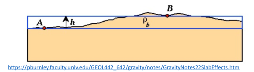
It is apparently shown in the figure above, gravity varies from A point to B point. There are two reason to explain the gravity variation. One reason is that A and B have the difference in topography. Another reason is the different amount of excess mass underneath cause the gravity variation from A to B. The excess masses would contribute more to the gravity anomaly.

The gravity variation caused by the excess mass underneath the B point can be approximated as a slab of material with thickness and density . Obviously, this description does not accurately describe the nature of mass below the point B, because the topography is not of uniform thickness and the density varies with location. But in this section, we assume the slab of material is regular (thickness ) and uniform (density ), the more detailed and complicated correction will be considered next.

3.2.4.2 Correct for excess mass: Bouguer slab correction

The method we used to correct (or, remove) the spatial variations in gravity that are due to the differences in the amount of the excess mass underneath each station (seeing figure above) is Bouguer slab correction, which is based on this simple slab approximation. We assume that the excess mass underneath B can be approximated by a slab of uniform density and thickness (seeing figure below).

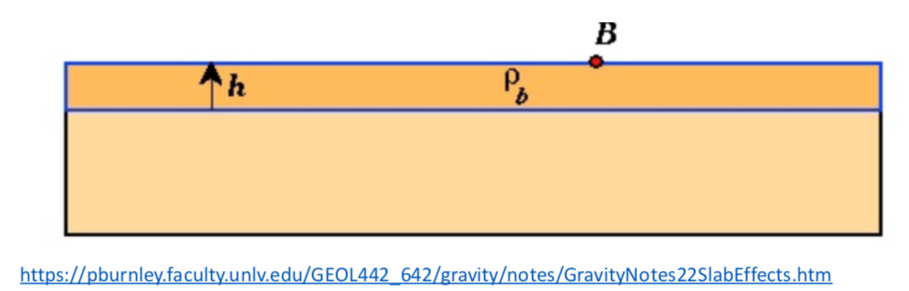
We remember gravity decays as a function of distance squared, so, the mass directly under the gravimeter and vary near areas contributes most to the measurements. The slab approximation, thus, can adequately describe how much of the gravity anomalies associated with excess mass.

In the Bouguer slab correction, the vertical gravitational acceleration associated with a flat slab can be simply written as .  Where is the density of the slab, is the elevation difference. is positive for observation point above the reference level and negative for observation points below the reference level. The negative sign of the Bouguer slab correction is make sense, because if an observation point is at a higher elevation, there is excess mass underneath. Our gravity reading, thus, is larger due to the excess mass, and we would subtract a gravity anomaly value to move the observation point back down the reference level.

In the Bouguer slab correction, we need to know the elevation of all observation points and the density of the slab used to approximate the excess mass. We currently use an average density for the rocks in the survey area. For a density of , the slab correction is about .

(https://pburnley.faculty.unlv.edu/GEOL442_642/gravity/notes/GravityNotes22SlabEffects.htm)

3.2.5 Terrain correction

3.2.5.1. The problem with Bouguer slab correction

In the previous section, we talked about how excess mass in the surface of the earth can lead to gravity variations. Having our stations be in different levels of topography can lead to changes in elevation and different amount of excess mass underneath them, which in turn leads to these gravity variations. For example, gravity measured on top of a mountain will be larger simply because there are more masses underneath it.  Recall that we can simplify the variations in topography by approximating it as a uniform slab with uniform thickness. This is only a rough approximation, and is also known as simple Bouguer correction. This rough approximation is adequate for simple gentle slopes, but there is a problem in Bouguer slab that arises if we have rougher topography. The problems can be classified into two:

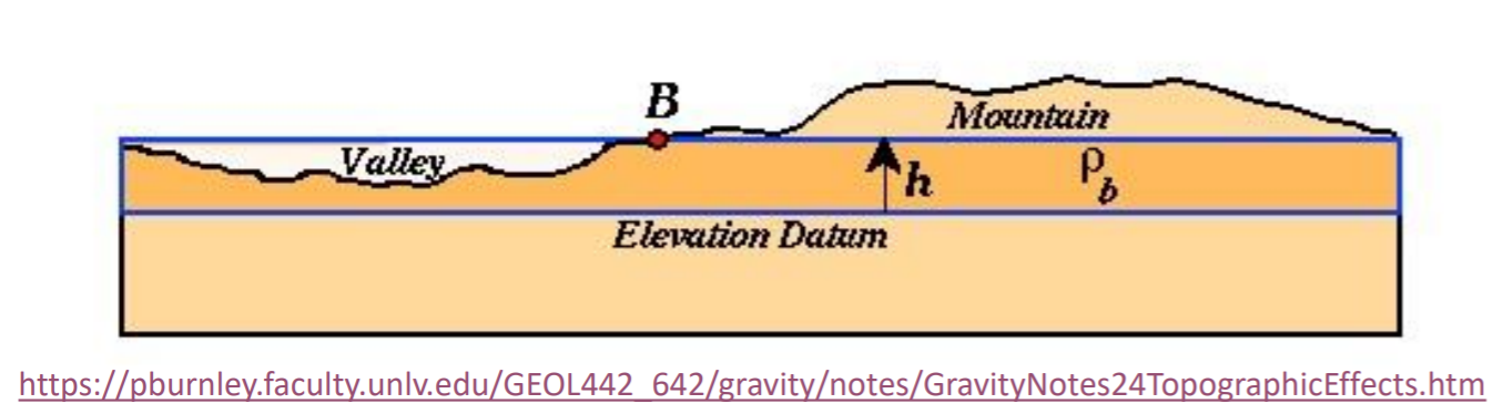
• Valleys

Consider the figure above and focus on the left-most part underneath the text that says “Valley”. We see that the area below the blue line (the Bouguer slab) in the left-most side does not account for the lack of mass. However, with our gravity correction scheme, you still subtract it with with the gravity due to the uniform slab. Thus, you will end up with overcorrection of gravity measurements near the valleys. The gravity measurement near the valley is already low even without the slab correction, but because we still subtract it in this process, you will end up with a lower gravity value than what you should have.

• Mountains

As before, consider the figure above, but focus on the right-most part above the text that says “Mountain”.  We see that the area above the blue line (the Bouguer slab) in the right-most side does not account for the excess of mass. With the gravity correction introduced in the previous section, you subtract the gravity measured at point B with the gravity due to the uniform slab. What’s missing is that it doesn’t take into account that the mountain will have its own gravitational attraction acting upon point B, which has an upward direction. This means that the gravity measurement that we measure in point B is supposed to be lower than it’s supposed to, due to the gravitational attraction of the excess mass above the slab. This means that we undercorrected our measurements.

The above factors poses a problem for our correction, which brings us to the need to do terrain correction.

3.2.5.2. Complete Bouguer Anomaly

Knowing the above factors, we must then find a way to account for the topography and terrain in our gravity correction. This can be done using terrain correction. Terrain correction is the small adjustment we make to our Bouguer slab correction to account for topography. This will produce the complete Bouguer Anomaly.  In other words, terrain correction is the gravity correction due to the excess/deficit of mass in the Bouguer slab, accounting for contribution from the valleys and mountains. In mathematical term, this can be expressed as:

In order to perform a terrain correction, we need a high resolution Digital Elevation Model (DEM). This tells us the x,y,z locations of all observation locations. We also need to estimate the densities of the terrain in order to calculate the gravity of terrain at all observation locations. However, this an be computationally expensive and time consuming.

Fortunately, digital topography maps are available worldwide. However, they are typically not fine-sampled enough for the near-zone terrain correction in areas of extreme topographic relief, or where high-resolution gravity observations are required. What we mean by near-zone terrain correction is corrections for topography located very close (within 558 ft) to a gravity station. If the topography is rough, there needs to be a very accurate elevation model. This requires very time consuming and expensive process.

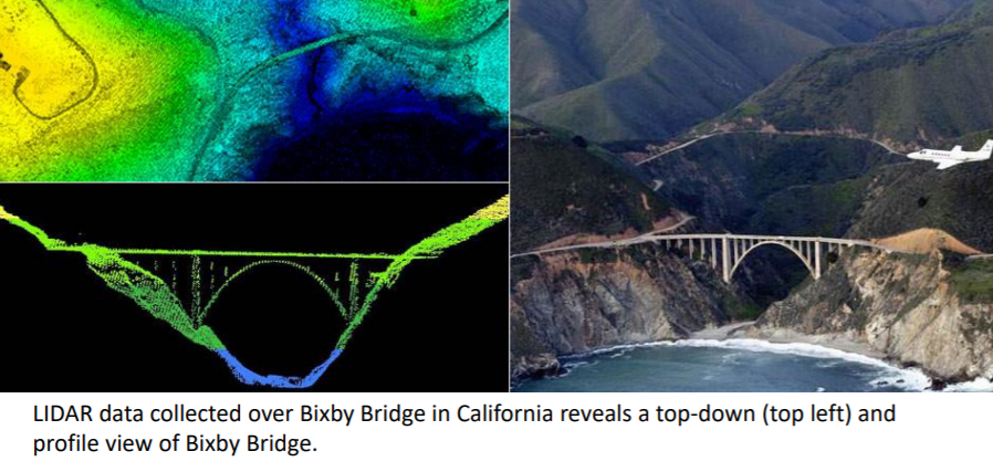
Thus we usually use LIDARs to quantify the topography of the area. LIDARs can be mounted into an airborne survey (helicopter, airplane, etc.). Airborne surveys can cover vast regional areas in a short period of time. The method is accurate to about a few millimeters (mm).

The excerpt below talks about the LIDAR in depth, which can be found from https://oceanservice.noaa.gov/facts/lidar.html.

3.2.5.3. Example of Terrain Corrections

Consider the following figure:

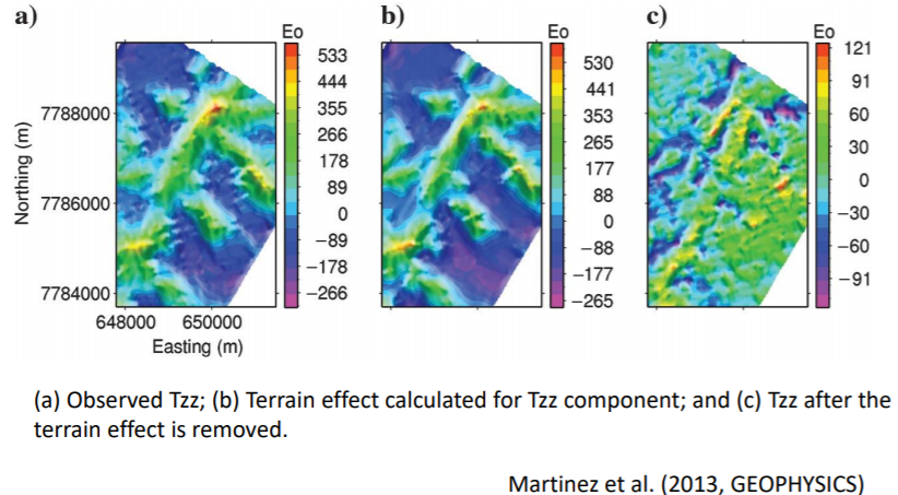
Figure (a) is the observed Tzz component of the gravity data while (b) is the terrain effect of the survey area. Notice that (a) and (b) are almost identical. What this indicate is that the contribution to the gravity data in (a) are mostly (or, completely) from terrain effects. This does not give us any important information about the subsurface density distribution. After applying terrain correction, we get Figure (c), which is the better data to be used for further interpretation processes (like inversion).

3.2.5 Hammer net

3.2.5.1. Terrain Correction History

Before the technological advancement that we have today, (that is, before we have LIDAR), researchers would need to manually calculate the terrain correction themselves. Terrain correction was first considered by Hayford and Bowie around 1912. Cassinis, Bullard, and Lambert in 1930s tackled the problem of how to estimate terrain correction. Hammer developed a practical approach for performing terrain corrections out to about 22km from the station. Bullard (1936) broke the terrain correction into three parts:

The first part is similar with simple Bouguer correction, which is also referred to Bullard A. This method approximates topography as an infinite horizontal slab of thickness equal to the height of the station above the reference ellipsoid or another datum plane.

The second part (Bullard B) is developed based on the curvature of the Earth, which reduces infinite Bouguer slab to a spherical cab of the same thickness with a surface radius of 166.735 km – 1.5 degree.

The third part (Bullard C) is terrain correction which takes undulations of topography into account. Topographic variations results in the upwards attraction of hills above the plane of the station and valleys below, which decrease the observed value of gravity, so both of these effects must be added to readings to correct for topography.

3.2.5.2 Hammer net

Hammer improved on the method of Hayford to simply terrain corrections. His “Hammer net” was widely used to make the terrain correction in past decades. This method involves compartmentalizing the area surrounding the measurement point using a template that is termed as Hammer net. Specifically speaking the Hammer net divides the area around a gravity station (shown in the figure below) using a template on the printed topographic maps.

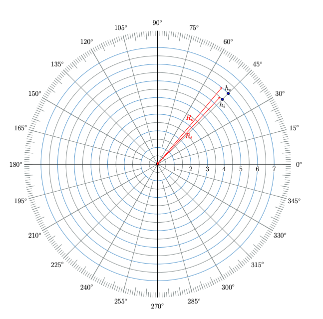
During the terrain correction process, for each gravity station (central red point in the figure above), a Hammer net is centered around it. The elevation of the centered station is determined through a known terrain model. The elevation difference, therefore, is estimated in each compartment by the Hammer net. The mathematical expressions of elevation estimation is following:

where is the station elevation, and are two known elevations of different compartment, is the elevation difference of compartments.

Clearly note that topography affects gravity data the most and in the innermost zone, so different inner zone correction is normally used and Hammer net correction is currently referred to an outer zone terrain corrections.

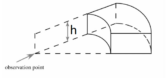
What is gravity effect of a radial component of a hollow vertical cylinder with a flat top?

   

where, :bulk density for the compartment, : angle subtended by the two radial lines bounding the segment, : inner radius, : outer radius.

Total terrain effect:

   

3.2.5.3. Complete Bouguer Anomaly

Complete Bouguer anomaly is associated with observed gravity, free air correction, slab correction, terrain correction and latitude correction, which reflects the subsurface density variations. The complete Bouguer anomaly can be expressed as:

where, is measured gravity, is free air correction, is slab correction, is terrain correction and is latitude correction.

Some Bouguer anomaly examples are shown below:

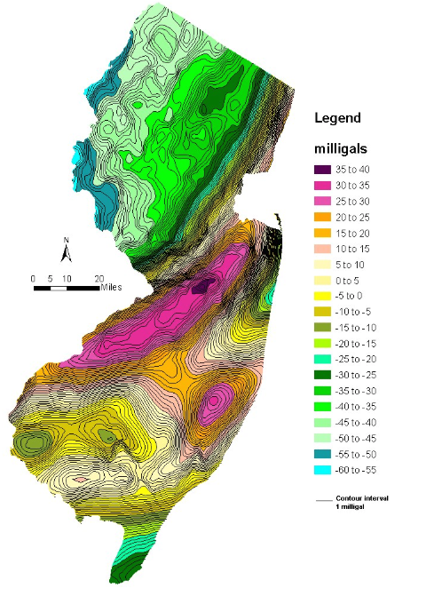
The figure shown above contains two GIS shape files of bouguer gravity contours, lines and polygons, at 1 and 5 milligal intervals respectively. The contours are based on gravity data in New Jersey and vicinity. The bouguer anomalies at 1 milligal interval range from a low of -58 milligals to a high of +37milligals. At 5 milligal intervals they have lows ranging from -55 to -60 milligals and highs ranging from +35 to +40 milligals.

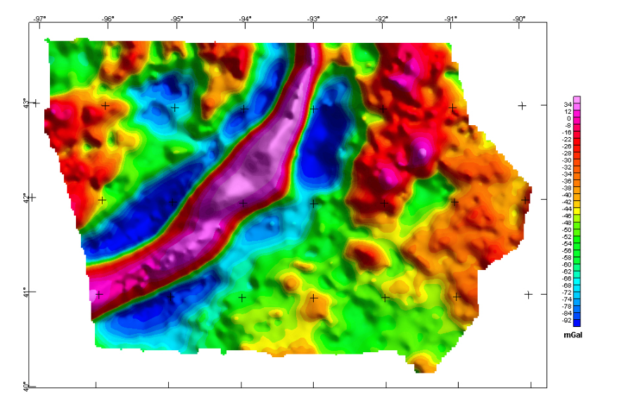
Bouguer gravity (figure shown above) reflects lateral density variations in the Earth. Positive anomalies (red color) occur in ares with average density greater than the Bouguer reduction density of 2.67 gm/cc, whereas negative anomalies (blue color) occur in areas of lower density. The highest anomalies are closely related to mid continent rift, which means something subsurface has really high density.

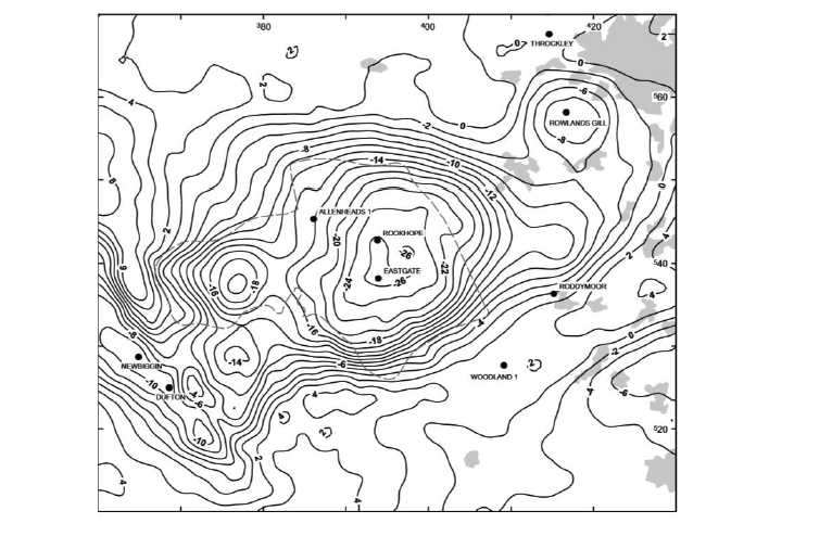
Based on the stations from the British Geological Survey national gravity databank. Contour interval = 2 mGal. Dashed line is the edge of the fluorite zone (after Dunham 1990). Grey shading indiates urban areas; black dots are selected boreholes (Figure 2 in Kimbell et al, 2010, The north Pennie batholith (Weardale Granite) of northern England – new data on its age and form).

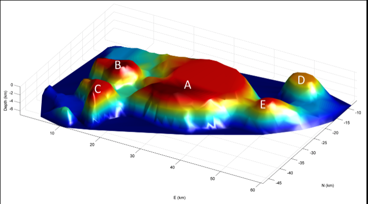
3D model of the North Pennine Batholith (aka the Weardale Granite), adapted from Kimbell et al. (2010). The North Pennine Batholith, also known as the Weardale Granite is a granitic batholith lying under northeast England, emplaced around 400 million years ago in the early Devonian. The batholith is composed of five plutons: A: Weardale Pluton B: Tynehead Pluton C: Scordale Pluton D: Rowlands Gill Pluton E: Cornsay Pluton.

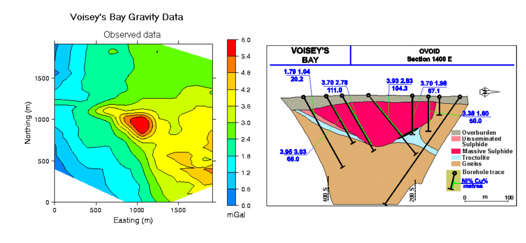
The figure above (left) is observed gravity data, the figure below (right) is geological model built based on drill hole data.

3.2.5.4. A Few More Examples

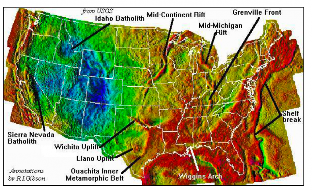
The negative (cold color)  in the West US in basin areas, the positive (warm color) in the East US in the mountain areas. The anomaly’s corresponding features are labeled in the figure above.

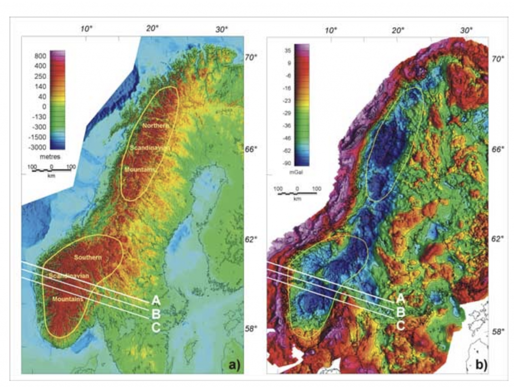
The observation from the figure above, the negative anomalies at location where the elevation is high.

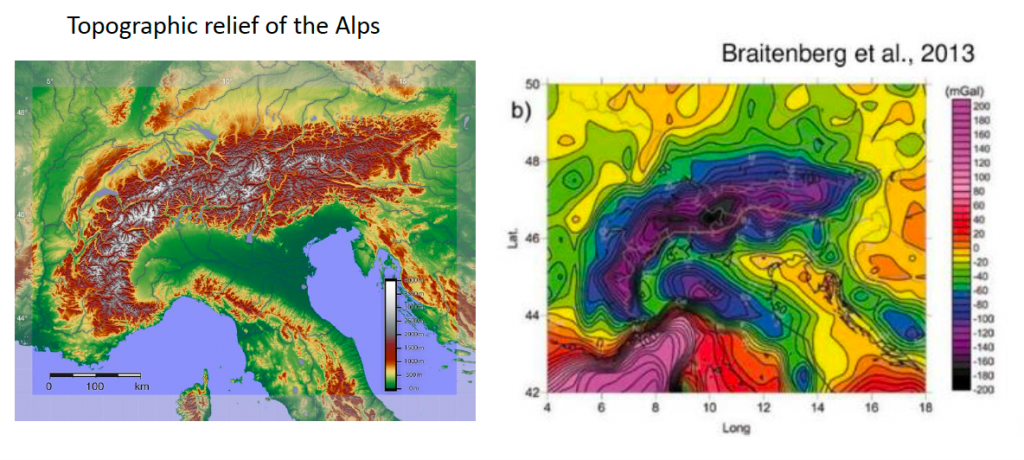
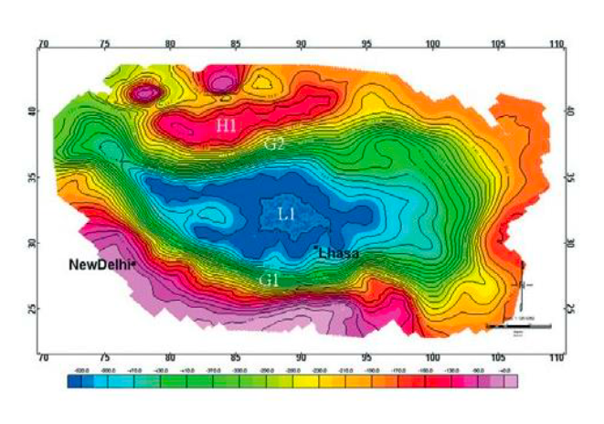
Bouguer anomaly map of the Himalaya and Tibet obtained from the satellite free air anomaly map (Shin et al., 2007) showing a major gravity low (L1 area) over Tibet and gradients G1 and G2 coincide with Himalayan. thrust and suture zone (ITSZ) and Altyn Tagh fault, respectively. The gravity highs, H1 are related to Tarim basin. We noticed that the gravity is lower over the Himalaya mountain. The trend is the Bouguer gravity  is generally lower over mountains.

3.2.6 Isostasy

3.2.6.1. Concept of Isostasy

In order to understand the concept of isostasy, we will first start by discussing Archimedes’ Principle. Archimedes’ Principle states that “A floating body will displace a volume of fluid whose mass is equal to that of the body.” Consider the following example of a cargo ship floating in the ocean:

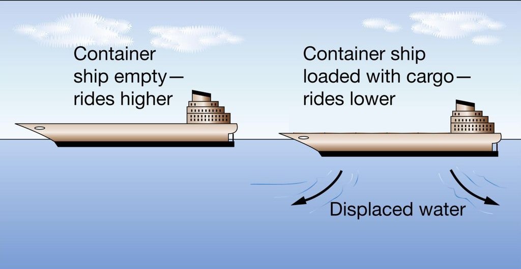
While the cargo ship is unburdened, it will float higher than after cargo is added. This is due to the increased density of the total body, which increases the water displaced and decreases the height that the ship floats at. In both situations, the ship is at hydrostatic equilibrium as stated by Archimedes’ principle, and isostasy is a geophysical way of defining the same concept. The word isostasy is derived from Greek and means “equal standing.” In geoscience, isostasy is the vertical positioning of the lithosphere so that the gravitational and buoyant forces balance one another. The body and fluid of Archimedes’ principle is the low-density lithosphere that floats on denser underlying asthenosphere in isostasy.

3.2.6.2. Hydrostatic Equilibrium

In the previous section, we briefly mentioned <strong>hydrostatic equilibrium</strong>, and we will further expand on the concept. Simply put, at hydrostatic equilibrium all mass involved in the system is in equilibrium and does not move. This means that the sum of all forces acting on a mass in this state must be zero according to Newton’s second law. Consider the following example of a block of rock located deep in the Earth:

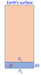
In the figure above, the block that we are considering is colored blue and has a density and length . In this case, the force on the top of the rock is . The force at the bottom of the rock is the sum of the force on top plus the gravity of the cube itself, and can be defined in the following equation:

Now, we will consider the following example of an iceberg at hydrostatic equilibrium:

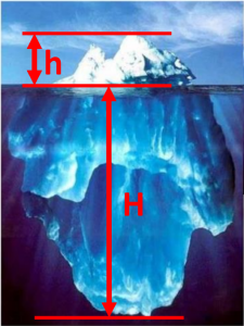
Suppose that the iceberg above sticks out of the water by a height and extends below the waterline at a length . By using the known densities of and , we can find the extent of based on using the following equation:

By substituting in the known densities of water and ice, we get:

At this point, we can define h as a ratio of H as area cancels out:

Now, imagine if we used a mountain instead of an iceberg in the example above. In this case, we would replace water with a sea of heavier mantle materials (e.g. olivine or pyroxene) but the same analysis applies if we assume that the mountain is also in hydrostatic equilibrium. However, we would apply a different term in geophysics as we would state that the mountain is in isostatic equilibrium or isostasy instead. Additionally, we must make the basic assumption that there is a depth at which the pressure due to the column of rocks above does not change laterally. This depth is called compensation depth or level.

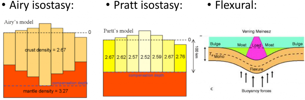
3.2.6.3. Isostasy

There are a couple of important concepts and assumptions related to <strong>isostasy</strong> that we must discuss. The first comes from the section above, and this is that there is a <b>compensation depth</b> or <strong>level </strong>at which pressure from a column of rocks above does not change laterally. Regions of high topography on a surface represents an excess of mass and pressure, which must be compensated at depth by a deficit of mass with respect to the surrounding region. Additionally, mountain belts are often also regions of thickened crust. This means that conversely, topographic depressions are matched by mass excesses at depth.

The figure below depicts three types of isostasy:

3.3. Magnetic MEASUREMENTS

Measurements of magnetic fields can be done using magnetic instruments. In this section, we will explain physics behind the instruments that we used to measure magnetic field, commonly used in geophysics.

3.3.1. Fluxgate Magnetometer

The fluxgate magnetometer was first invented in 1936 before WWII and was mostly used to detect submarines (which are metallic, and therefore would produce magnetic signals). The fluxgate magnetometer was also the type that was used to prove the theory of plate tectonics. As we have explained in the previous section, the evidence of plate tectonics and seafloor spreading were found from the magnetic measurements near mid-ocean ridges, that form what we call as “magnetic stripes”.

3.3.1.1. Concepts

Before going through the details on how Fluxgate Magnetometer works, let us review some concepts in magnetics that will be useful in this section. First concept is magnetic susceptibility (), a dimensionless property. If we  assume an inducing field H (for example the earth’s magnetic field at the geographic region) that is applied to a magnetic material, then it will produce an induced magnetization M in the material. This is mathematically expressed as:

From the linear relationship above, theoretically we can say that the magnetization (M) increases if we increase the inducing field (H). However, some magnetic materials under the influence of an external magnetic field, will reach a state where an increase in the external magnetic field H does not increase the magnetization of the materials further. In other words, the magnetic flux levels off as you increase the external field, and continues to increase at a very slow rate due to vacuum permeability. This phenomenon is called magnetic saturation.

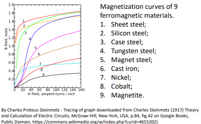
From the above picture, we see that different magnetic materials will have different curves associated with the relation between H field (inducing field) and B field (induced field, equivalent to M). Some curves saturate at a slower rate than others, and this depends on the materials.

Now that the above concepts are explained, we can move on to explaining more about the physics behind fluxgate magnetometers.

3.3.1.2. Instrument Parts

Primary Coil

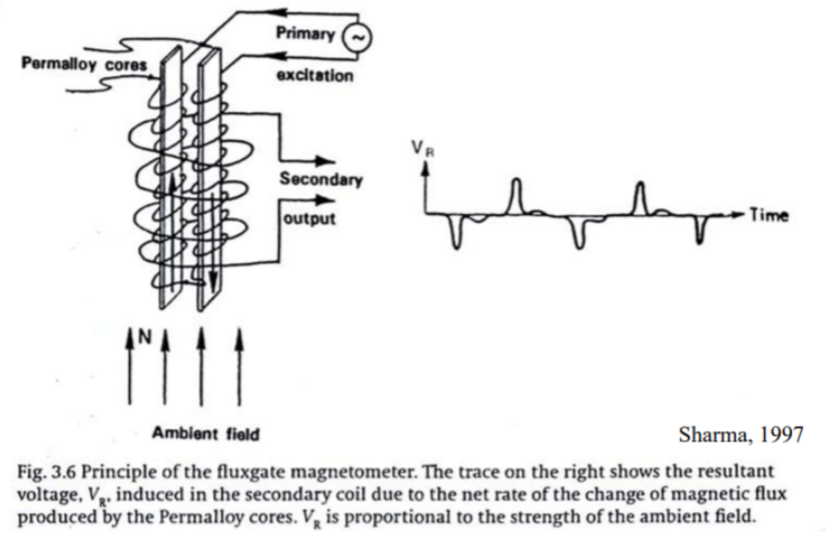
A fluxgate magnetometer can be explained by the following diagram:

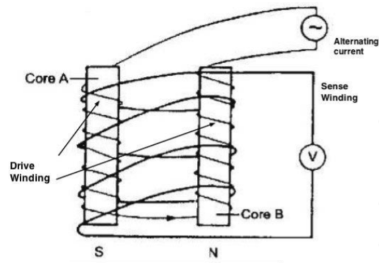
We can see that the magnetometer is made off two cores that are made off ferromagnetic materials, labelled as Core A and Core B. These cores are placed next to each other and have two loops surrounding it. One loop is called the primary coil/sense coil and has an AC (alternating current) going through it. This one coils around core A and core B as the following picture:

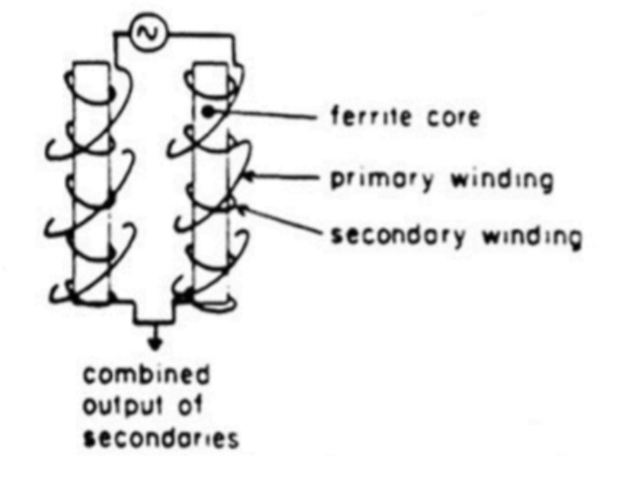
The AC current generates magnetic field H and gets the two cores magnetized. However, their magnetization varies with time. This is because AC current varies with time and thus the magnetic field H also varies in time. Notice that the primary coil is wound in the opposite senses around the two cores (ex: Core B is wound such that the magnetic field direction goes down, and core A is wound such that the magnetic field direction goes up). Because the inducing fields H are in the opposite direction in these two cores, therefore, these two cores get magnetized in opposite directions.

Secondary Coil

The other coil that wounds through both core A and core B is used to measure the voltage in the two cores (indicated by the letter ‘v’ in the schematic of the fluxgate magnetometer). This is the secondary coil and it measures the voltage using Faraday’s Law. To understand this, we introduce the concept of electromotive force (emf). It is the force that drives currents to flow in a wire or in a conductive body, with unit of volts. It can be expressed mathematically as such:

Where is the magnetic flux. Any change in magnetic flux induces an emf/voltage. This process is called electromagnetic induction. An emf, when applied to a conductor, generates current.

3.3.1.3. Measurements

Knowing that the secondary coil measures the emf, and that the changes in current throughout time also causes the magnetization to change throughout time, let us examine the following figure:

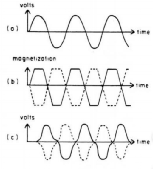
From the above picture, (a) is the emf from the AC current that changes in time. This in turn changes the magnetization of the cores as we see in (b), where the dash line is from core A and the solid line is from core B. Notice that the magnetization saturates to a flat line after a certain amount of time, and changes with the alternating current. In addition, (c) is the measured emf from the change in magnetization between core A and core B. Notice that if we add the dash line (emf from core A) and solid line (emf from core B), the summation will result in zero. Thus, the sum of the voltages from the two cores is zero if there is no external magnetic field.

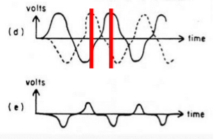
In the presence of an external field, for example, if this two-core system is placed in the earth’s magnetic field, then the sum of the voltages between the two cores is non-zero. Let’s look at the figure below:

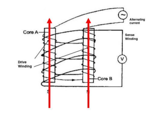
In this case, the earth’s magnetic field is represented as the red line pointing upwards. The total magnetic field applied to core A increases, and thus the magnetization reaches saturation earlier. The total magnetic field applied to core B thus decreases (opposite directions) and the magnetization reaches saturation later than in core A. Consequently, the voltages from these cores will have a phase shift, producing a non-zero summation of the voltages.  This phase shift due to the external magnetic field is captured in the voltage measurements as the following figure (d), and the summation of voltage can be seen in figure (e).

In some systems, a third coil which passes a direct current is wrapped around the entire system. This produces a magnetic field that offsets the earth’s field. When the output of the secondary coil is reduced to zero, then the DC field is exactly equal and opposite to that of the earth’s magnetic field. Thus, by monitoring the DC required to maintain zero secondary output, variations in the earth’s magnetic field can be measured.

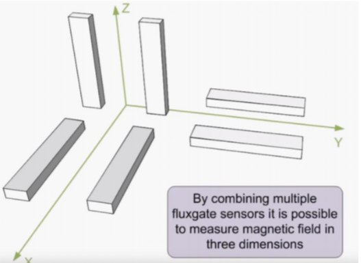
Knowing how a fluxgate magnetometer works, the two-core system can be put in three directions in order to get the three components of the magnetic field (Bx, By, Bz).

Source: https://www.youtube.com/watch?v=_5d0qz_umuE

A fluxgate can measure the component of the earth’s magnetic field in the direction of the axis of the system. By purposely pointing the axis into a direction, we can measure any component of the earth’s magnetic field. Thus, to measure the total field, we can either:

1. Measure the three component using three mutually perpendicular system
2. Orient a single system in the direction of the total field

3.3.2. Proton Precession

3.3.2.1 Atomic nucleus and proton

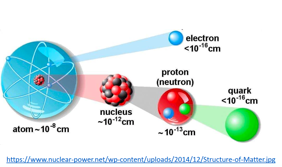
Proton is the fundamental part of the proton precession magnetometer. So, firstly, we briefly recall the atomic nucleus and proton.

The atomic nucleus is the small, dense region consisting of protons and neutrons at the center of an atom. An atom is composed of a positive-charged nucleus, with a cloud of negative-charged electrons surrounding it, the nucleus and electrons bound together by electrostatic force. Almost all of the mass of an atom is located in the nucleus, with a very small contribution from the electron cloud. Even though, the nucleus contains almost 99.9% of the mass of an atom but only occupies a volume whose radius is 1/100,000 the size of an atom. Protons and neutrons are bound together to form a nucleus by the nuclear force.

3.3.2.2 Precession

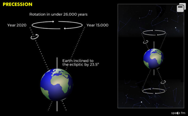
Precession is a change in the orientation the rotational axis of a rotating body. In other words, if the rotation axis of a body is itself rotating about a second axis, that body is said to be precessing about the second axis.

The Earth rotates on its axis but has a slight ”wobble or ‘oscillation’ to be precise like a spinning top. This wobble takes approximately 26,000 years and has implications for how we view and measure the stars over a long period. The process is known as precession of the equinoxes or axial precession. Main reason for precession of Earth is that Earth is not a perfect sphere and is an oblate spheroid, it is slightly wider at the equator. The Sun and Moon have a gravitational influence on Earth and this combined with the Earth’s bulge causes a wobble in the Earth’s tilt.

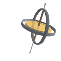
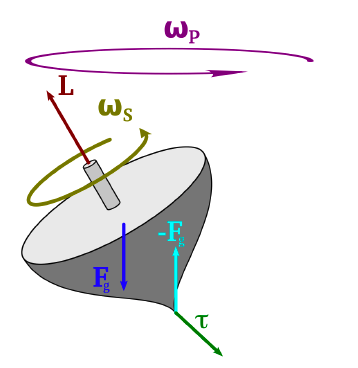
Here, we introduce the precession of a spinning top. A rapidly spinning top will precess in a direction determined by the torque exerted by its weight. The precession angular velocity is inversely proportional to the spin angular velocity, so that the precession is faster and more pronounced as the top slows down. Spin a top on a flat surface, and you will see it’s top end slowly revolve about the vertical direction, a process called precession. As the spin of the top slows, you will see this precession get faster and faster. It then begins to bob up and down as it precesses, and finally falls over.  In other words, any rotating objects (i.e., with an angular momentum) can undergo precession under the influence of a torque.

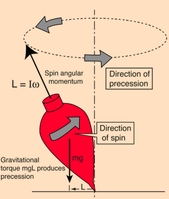
Precession of a top

The torque caused by the normal force and the weight of the top causes a change in the angular momentum in the direction of that torque. This cause the top to precess.

The mathematical equation for precession of a top is:

   

where, : torque, : angular momentum.

 

It is important to note that if an object has an angular momentum  (i.e.,  it is rotating), and if an external torque exists, the object will precess.

3.3.2.3 Precession of a proton

A proton has an angular momentum, resulting from spin of a proton. Just like a top has an angular momentum. The more specific information refer https://physicsworld.com/a/the-spin-of-a-proton/.  Objects possessing momentum tend to maintain their motion unless acted up by an external force. In our cases, the gravity can create a torque. For magnetic data acquiring, a torque can be created by an external magnetic field. The equation is below:

where, : torque, : magnetic dipole moment, : external magnetic field, : angular momentum vector.

Therefore, a proton will precess. The external field with angular frequency knowns as Larmor frequency.

where, : angular frequency in radians / sec, : a particle-specific constant.

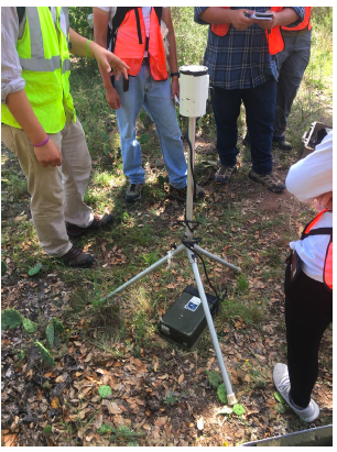
3.3.2.4 Proton precession magnetometer

The proton magnetometer, also known as the proton precession magnetometer uses the proton precession to measure the variation in the Earth’s magnetic field. The cylinder at the top (white) contains hydrogen-rich fluid (e.g., kerosene, decane, water). There is also a solenoid. When direct current flows in the solenoid, a strong magnetic field is created. The protons align themselves with that field. Then the current is interrupted, and as protons realign themselves with the ambient magnetic field. The external Earth’s field creates a torque, and causes the protons to precess and they precess at a frequency that is directly proportional the magnetic field.

3.3.3. Akali Vapor

3.3.3.1. Basic Concepts of Alkali Vapor Magnetometers

The easiest way to understand Alkali Vapor Magnetometers is to start by deconstructing its name. Alkali is fairly simple, and refers to alkaline metals such as cesium, potassium, and rubidium that can be used in the construction of Akali Vapor Magnetometers. The magnetometer contains an alkali metal within a cell or chamber that will continuously heat the metal until it reaches a gaseous form. In the case of cesium, this vapor can be produced at temperatures ranging from approximately 45 to 55 degrees Celsius. The vapor is important as these magnetometers operate based on splitting electron energy levels in alkali metals by the Zeeman effect.

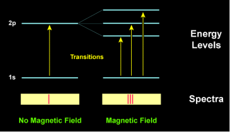
3.3.3.2. Zeeman Effect

In order to explain the Zeeman Effect, we will need to delve a bit into quantum mechanics. When an external magnetic field is applied to an atom, its atomic energy levels are split into a large number of levels. Under a continuous spectrum of light, spectral lines are distinct lines resulting from either light emission or absorption by atoms or molecules which form against the continuous background. These lines can be used as “fingerprints” to identify molecules or atoms, but are split into multiple components of slightly different frequencies when under the influence of a magnetic field. This is called the Zeeman Effect and was first observed by Dutch physicist Pieter Zeeman who shared the 1902 Nobel Prize in Physics with Hendrik Lorentz for this discovery.

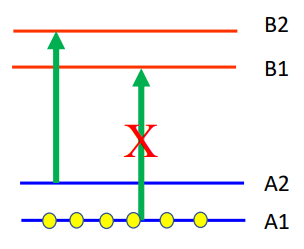
The figure below shows the splitting of energy levels and the changes to the light spectra under a magnetic field:

We will now do a deeper dive into the physics behind the Zeeman Effect. We will start with the atomic energy levels of an atom or molecule when there is no magnetic field.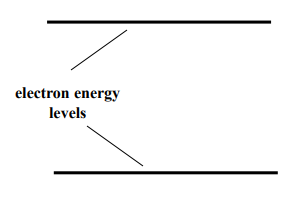

When an external magnetic field is applied, the atomic energy levels will separate. The figure below labels the separated energy levels as A1, A2, B1, and B2.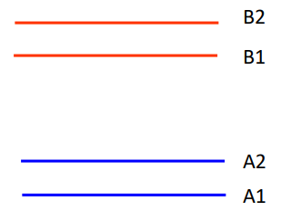

The energy gap between energy levels such as A1 and A2 is determined by the strength of the applied magnetic field. In an Akali Vapor Magnetometer, a beam of light with a frequency that corresponds to the energy gap between A2 and B2 can be used to irradiate the akali vapor. Electrons in the vapor at energy level A2 will absorb the energy from the beam and move to the higher energy level of B2. Additionally, the beam can be manipulated so that it does not contain any frequencies corresponding to the energy gap between A1 and B1. This process is called polarization.

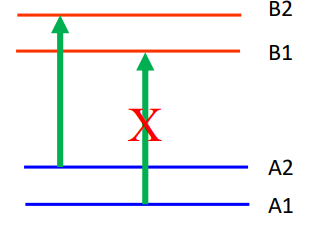
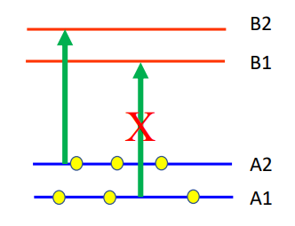
In other words, after polarization electrons can only jump from A2 to B2 but cannot jump from A1 to B1. This means that electrons from A2 will all jump to B2, but B2 is at a higher energy state and therefore unstable. This means that energy will be released and the electrons will fall back down to either A1 or A2. This process of rising and falling atomic energy states will continue in a loop until all electrons eventually settle at A1. This process of overpopulating one energy level is known as optical pumping. At this point, the photons from the light beam will pass through the magnetometer’s chamber with no energy loss. The vapor is therefore registered as transparent, and a photosensitive detector in the magnetometer will register a maximum current.

At this point, an RF (radio frequency) signal that has a frequency corresponding to the energy gap between A1 and A2 can be applied. This will lead some of the electrons to jump up to A2 which will absorb the photons from the light beam once again. The photosensitive detector will measure a decrease in current at this point. Unfortunately, the exact frequency of the desired RF frequency is unknown, so a varying RF signal is applied to sweep through a range of possible frequencies. This frequency is related to the energy gap which is determined by the strength of the magnetic field according to Zeeman splitting.

This means that by measuring the RF frequency accurately, an alkali vapor magnetometer can determine the strength of a magnetic field.

3.3.3.3. Alkali Vapor Magnetometer

When compared to the proton precession magnetometers mentioned previously, an alkali vapor magnetometer is an order of magnitude more sensitive. The sensitivities reported can range from as small as 0.001 to 0.01 nT. This is compared to a proton precession magnetometer which has an accuracy ranging from 0.1 to 1 nT. The most commonly used alkali vapor magnetometers are cesium vapor and potassium vapor magnetometers.

It is important to note that the magnetometers that we have mentioned so far are scalar magnetometers. There are also vector magnetometers, such as Fluxgate and SQUID (superconducting quantum interference devices). A fluxgate magnetometer has a sensitivity of about 0.1 to 1 nT like the proton precession magnetometer, but a SQUID magnetometer is far more sensitive than any of the other magnetometers that we have mentioned so far.  It has a sensitivity of nT, and can measure the three-components of magnetic field along with its gradients.

3.4. Magnetic Data processing

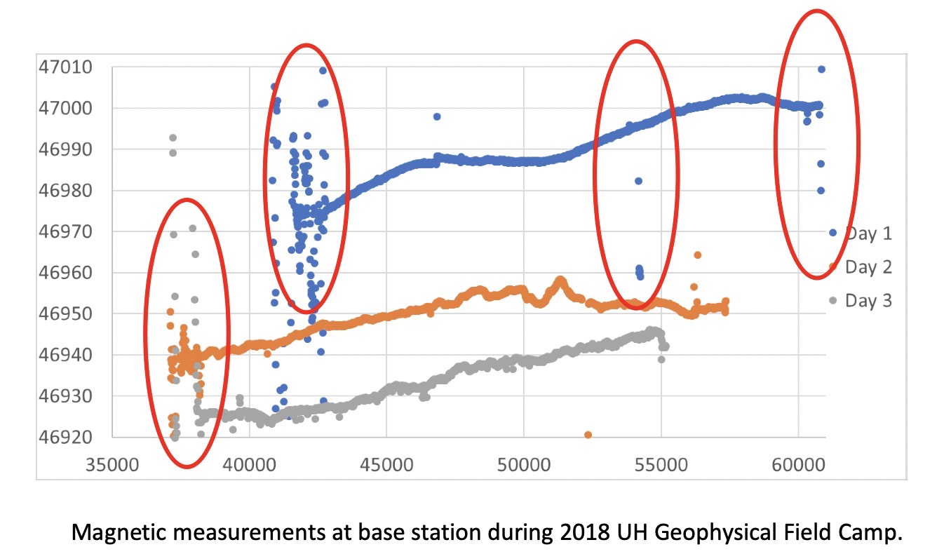
Like raw gravity data collected in the field, magnetic data also needs some necessary corrections before being interpreted. As data are shown in the graph above, the blue, orange, gray dots are magnetic data recorded as the base station through the day 1, 2, and 3; the horizontal axis represents the time, the vertical axis denotes the magnetic data in . The red ellipses grouped data with a large number of noises.

The data measurements are taken with varied spatial locations in order to cover the study area, meanwhile, the recorded data are taken at different time periods of a day, which is reflected from the linear trend in the data shown in the above graph. Therefore, we need to remove the time variation effect, to left only the spatial variations due to the local geology we are interested in.

3.4.1 Diurnal correction

The time variation effect removal from the magnetic data is called the Diurnal correction, which is to take consideration of the magnetic field changes due to the solar activities and their interaction with the ionosphere and magnetosphere. Because these changes have nothing to do with subsurface geology, therefore, they need to be removed from the raw measurements to enhance the signal from the geology features.

Usually, in data acquisition, one magnetometer was fixed at the base station to take continuous measurements of the magnetic field, say, every 10 seconds; while another magnetometer will be carried to the field to record at various locations.

3.4.2 IGRF subtraction

After subtracting the temporal variations of the magnetic field, what’s left is the variation due to the normal Earth, and the materials deep in the core. Therefore, the International Geomagnetic Reference Field (IGRF) subtraction will be taken, in order to subtract the background magnetic field produced by the Earth’s deep interior materials, so that, we can only focus on magnetic anomalies from the crust.

In general, the vertical gradient varies from approximately 0.03 at the poles to 0.01 at the magnetic equator, while the longitude variation is rarely greater than 6 . Therefore, elevation and latitude corrections are generally unnecessary.

To do this IGRF correction, we can input the longitude and the latitude of the measurement location into a mathematical model of the Earth magnetic field. After the subtraction, what’s left in the data is from the local geology.

Moreover, besides the two corrections mentioned above, do we also need to consider the terrain effects in the magnetic data? The answer is no, in general. However, in some special cases, terrain effects can be significant. For example, terrain effects can be as large as 700 at steep slopes (e.g., 45 degrees) on only 10 m extent in formations containing 2% magnetite. In such cases, terrain correction should be done. However, this correction requires us to know the magnetic source bodies in the terrain and be able to model their magnetic effects, which is very hard to achieve! Moreover, crustal magnetization can vary by several orders of magnitudes at essentially all spatial scales. Thus, we generally do not do terrain correction. The effects of terrain are often left to the modeling and interpretation stage.