2 Chapter 2: Potential Field Theory
Jiajia Sun; Xinyan Li; Felicia Nurindrawati; Xiaolong Wei; and Kenneth Li
2.1 Fundamental concepts
In this section, we will look at a few fundamental concepts that are highly relevant to the gravity and magnetics. These concepts include field, work, conservation field, and potential.
2.1.1 Field
A field is a set of functions of space and time. Mathematically, a field can be summarized as follows:

There are two types of fields that we are concerned about within this course, material fields and force fields.
A few examples of material fields include
- A density field that describes the density value at each point of a material (e.g., the Earth) at a given time;
- A porosity field that describes the porosity value at each point of a material (e.g., a reservoir) at a given time;
- A temperature field that describes the temperature value at each point of a material (e.g., a turkey) at a given time.
As you can tell, a material field describes some physical property of a material at each point of the material and at a given time.
The second type of field that is relevant to this course is the force field. A force field describes some kind of forces that act at each point of space at a given time. Some examples of force fields include
- Gravitational field that describes the gravitational force that acts at each point of space at a given time;
- Magnetic field that describes the magnetic force that acts at each point of space at a given time.
Moreover, the field can also be classified as either a scalar field or a vector field.
A scalar field is a single function of space and time, mathematically denoted by
For example, a scalar field could be:
- displacement of a stretched string;
- temperature of a volume of gas;
- density within a volume of rock.
A vector field is a vector function of space and time, which can be written as
 or
or 
Since it is a vector function, the vector field is characterized by three functions of space and time. Mathematically, these functions can be written as:


Examples of vector fields including:
- flow of heat;
- velocity of a fluid;
- gravitational attraction of a mass.
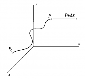
To visualize vector fields, we can use field lines, aka lines of flow, or lines of force. These are lines that are tangential to the vector field at every point. Therefore, scalar fields do not have field lines. Since field lines are tangential to the vector field at every point, it follows that small displacement along a field line must have  ,
,  , and
, and  components proportional to the corresponding , , and components of the field at the point of its displacement. This can be proved by the illustration and derivations in the following.
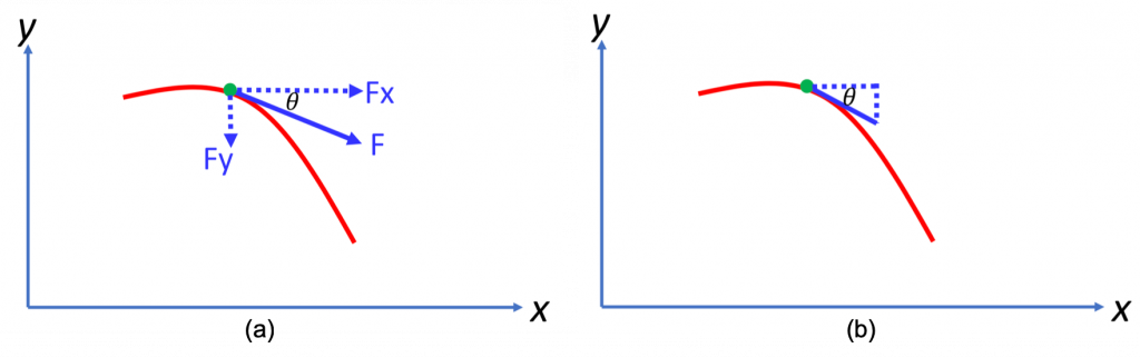
From the above figure (a), it is straightforward to derive the equation
(1) 
Now, let’s forget about the force in figure (a). Just consider this red curve in figure (b) as a function  . Then at the same green dot location, what is the derivative of the function at this point? According to the definition of derivative evaluated at a point, we can write the following equation:
(2) 
Since  is common for both equation (1) and (2), we can then link these two equations by
(3) 
Rearranging equation (3), we will have:
(4) 
Further extending this equation to 3D space, it can be mathematically expressed as:
(5) 
Therefore, if a vector field  is continuous, its field lines can be mathematically described by the differential equation (5).
Exercises
Find the gravitational attraction of a uniform sphere of mass M, centered at point Q, and observed outside the sphere at point P, through the given equation of

where  is a constant,
  is the distance from Q to P, and
  is the unit vector directed from Q to P.
Let Q be at the origin. Use the differential equation to describe the gravitational field lines at each point outside the sphere.
2.1.2 Work
Let us recall what we have learned in college Physics courses, the work is defined as the product of force and distance. For example, as the cartoon image shown below, assuming a constant force acting on the airplane from time equals zero to some distance  after some time interval, the work done on the airplane, denoted by
  , can be mathematically calculated by:

For this simple example, the force is assumed to be along with the same direction of the displacement. The unit of work is Joules, which is equal to Newton – meter is the SI unit system.
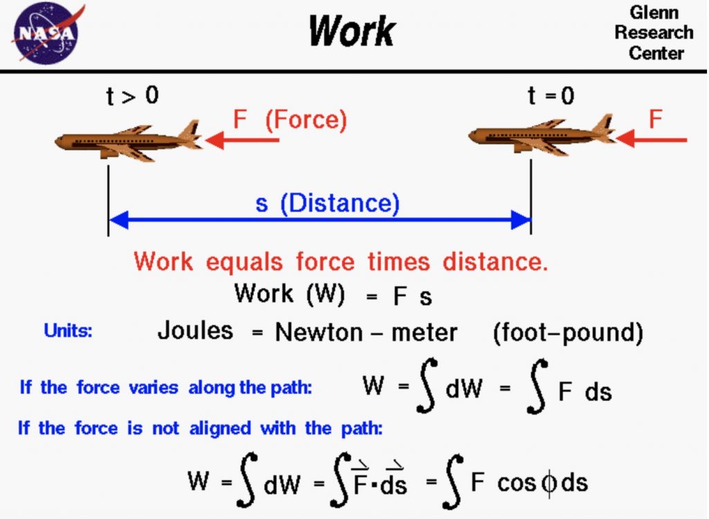
However, if the force is no longer a constant value, but varies along the displacement, then the work is the integrated value of the force along the distance. Its math expression is as follows:

Moreover, for the vector quantity force, if the force direction is not parallel with the moving path, then work is the integrated value of the force component along the direction of the path. Let the angle between the force and the displacement be  , the work can be mathematically calculated by the following:

Let us consider a more realistic example, illustrated by the figure below. A particle of mass  moves from position
  to
to  under the influence of force field . What is the work done by the force field in this example?
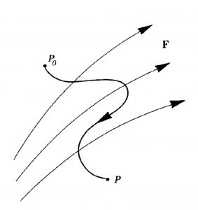
In this given example, the force direction is not aligned with the particle displacement path. Therefore, the work required to move the particle from position to is the integrated value of the force component along the path direction, which can be mathematically represented as the following:

2.1.3 Conservative field
In general, the work depends upon the path taken by the particle. However, for some fields, the work is independent of the path of the particle. These fields are said to be conservative. Please keep in mind that, since we are talking about work and force, the fields we are talking about are vector fields, which are vector functions of space and time.
Now let us consider another example of work done in the conservative field. The scenario is illustrated in the figure below. Assuming a particle of mass moves through a conservative field, first from position to in an irregular path, then parallel to the axis with an additional small distance  . What is the work?
We can deal with work done from position to  by summing the work from to with work from to
  . Its math expression is as follows:
(1) 
Rearranging the terms in equation (1), we will have equation (2) below:
(2) 
Since the path from position to is parallel with axis, we can calculate the work done along this path segment by the integration as follows:
(3) 
Therefore, combining equation (2) and (3), we will have the following equation:
(4) 
By applying the Mean value theorem to the integral calculation, equation (4) can then be written as follows:
(5) 
Dividing both sides of equation (5) by the small distance , we will have the new equation as below:
(6) 
Now if we make approach 0, that is,
(7) 
For the left-hand side of the equation (7), the limit is defined to be the derivative of the function work  evaluated at point ; the right-hand side of the equation is defined to be the force component along axis. Therefore, equation (7) can then be expressed as follows:
(8) 
Similarly, we can repeat the same derivation for the and directinos, and obtain the following:
(9) 
In a more compact form, equation (9) can then be summarized as follows:
(10) 
How to interpret this equation? It can be explained in the following aspects:
- gradient of work (or, work functino) (i.e., the left-hand side of equation (10)) is equal to force (i.e., the right-hand side of equation (10));
- derivative of work in any directino is equal to the component of force in that direction (e.g., the component in this example);
- the vector force field is completely specified by the scalar field .
In brief summary so far, a conservative field, , is given by the gradient of its work function, . Or vice versa, any vector field that has a work function satisfying the relation  is conservative.
2.1.4 Potential
Potential of a vector field is defined as the work function (or its negative). Its math representation is as follows:

Usually, potential is defined at the infinity to be 0. And the potential at point is defined as

2.1.5 Equipotential surface
As the name implies, an equipotential surface is a surface on which the potential remains constant. That is

Let us suppose  is a unit vector that is tangential to an equipotential surfacee of , which is illustrated in the figure below.
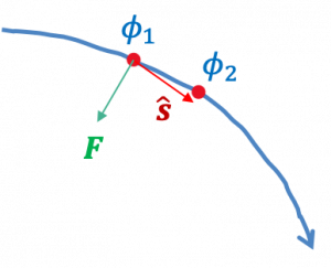
Since the potential is constant at any point along the equipotential surface, then we will have

That is, the dot product of a unit vector with force field is equal to the derivative of the potential with respect to the unit vector,  . We can think the derivative definition as the finite difference, i.e., the potential difference between
  and
and  , and if the distance between them is approaching to 0, then the derivative equals 0. Therefore, the dot product of the unit vector with force field equals 0.
According to the math definition of dot product between two vectors, since the dot product of the unit vector with force field equals 0, then the unit vector is perpendicular to the force field. That is,

Therefore, the field lines at any point must be perpendicular to their equipotential surface. Conversely, any surface that is everywhere perpendicular to all field lines must be an equipotential surface. And no work is done when moving a test particle along an equipotential surface.
2.2 Helmholtz Decomposition
Helmholtz theorem can be expressed as the following equation:
![\[F = \nabla \phi + \nabla \times A\]](https://uhlibraries.pressbooks.pub/app/uploads/quicklatex/quicklatex.com-e91eb6692117f76f40c20558c0c6c345_l3.png "Rendered by QuickLaTeX.com")
This basically says that “any vector field (F) can be represented as the gradient of a scalar () and the curl of a vector (A)”. The details and proof behind the above equation will be explained in this section.
Recap on important concepts
Before moving on to the next part, make sure that you understand the following points in order to make it easier to understand the derivation of the Helmholtz theorem.
- The difference between gradient (
 ), divergence (
 ), and curl (
 )
)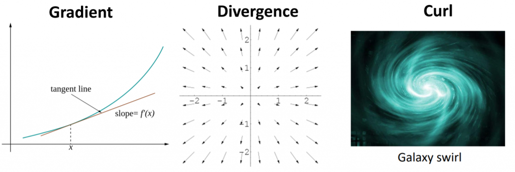
- The curl of a conservative field (such as gravity field) is always zero

- The divergence of a curl is always zero

Please review the previous section if the points above does not make sense to you.
2.2.1. Laplace Operator
Laplace operator is defined as the divergence of the gradient of a function. It can be expressed using the following expression:
![\[\nabla . \nabla f\]](https://uhlibraries.pressbooks.pub/app/uploads/quicklatex/quicklatex.com-f32a879a4f55e30753ae844d5f1b5860_l3.png "Rendered by QuickLaTeX.com")
where f is the function. To mathematically understand what the Laplace operator means, let us consider a Cartesian coordinate system with 3 directions (x,y,z). Thus the above expression can also be expressed as such:
![\[\nabla . \nabla f = \frac{\partial^2}{\partial x^2} + \frac{\partial^2}{\partial y^2} + \frac{\partial^2}{\partial z^2}\]](https://uhlibraries.pressbooks.pub/app/uploads/quicklatex/quicklatex.com-8ae7e30d0e3668b2444d66a7cf3937c9_l3.png "Rendered by QuickLaTeX.com")
The Laplacian (Laplacian operator) notation can also be further simplified as  or
or  .
.
Thus the Laplacian operator itself in a Cartesian coordinate can be written as:
![\[\nabla^2 = \frac{\partial^2}{\partial x^2} + \frac{\partial^2}{\partial y^2} + \frac{\partial^2}{\partial z^2}\]](https://uhlibraries.pressbooks.pub/app/uploads/quicklatex/quicklatex.com-8cda6b38361f1dfd3240d938701b1993_l3.png "Rendered by QuickLaTeX.com")
An Example of a Laplacian
One example of a Laplacian is the Laplacian of an inverse distance, which is 0 everywhere except at  . The Laplacian of the inverse distance can be expressed as such:
![\[\nabla^2(\frac{1}{|r-r'|}) = -4\pi\delta(r-r')\]](https://uhlibraries.pressbooks.pub/app/uploads/quicklatex/quicklatex.com-0e90f2e82edff4db762eee764168f152_l3.png "Rendered by QuickLaTeX.com")
The delta function ( ) represents the following:
![\[\delta(r-r') = \begin{cases} \infty, \tab r=r' \\ 0, \tab otherwise \\ \end{cases}\]](https://uhlibraries.pressbooks.pub/app/uploads/quicklatex/quicklatex.com-99c6417cc265375dbc2e978809d90936_l3.png "Rendered by QuickLaTeX.com")
The derivation of this function will be covered in the next section.
2.2.2. Poisson’s Equation
Poisson’s equation is expressed as the following:
![\[\nabla^2 \phi = f\]](https://uhlibraries.pressbooks.pub/app/uploads/quicklatex/quicklatex.com-306db642cc76bf779b55226474b99944_l3.png "Rendered by QuickLaTeX.com")
Usually, f is given, while we want to find what is. The solution to the above equation can be expressed as an integral over all of space:
![\[\phi = -\frac{1}{4\pi} \int \frac{f}{r} dv\]](https://uhlibraries.pressbooks.pub/app/uploads/quicklatex/quicklatex.com-792e40ef1d7fc54f826e0a0aa8af12b5_l3.png "Rendered by QuickLaTeX.com")
2.2.2.1. Example of Poisson’s equation in gravity application
The following is an example of Poisson’s equation:
![\[\nabla^2 \phi= -4\pi\gamma \rho\]](https://uhlibraries.pressbooks.pub/app/uploads/quicklatex/quicklatex.com-459ca44921c3301ceef6a949ea1e32c1_l3.png "Rendered by QuickLaTeX.com")
Usually, we know what  is and we want to know . The solution to the above equation can be expressed as such (just replace f with
  ):
):
![\[\phi = -\frac{1}{4 \pi} \int \frac{f}{r} dv\]](https://uhlibraries.pressbooks.pub/app/uploads/quicklatex/quicklatex.com-aafbe6652f1d7078e47328a814ac32c6_l3.png "Rendered by QuickLaTeX.com")
![\[\phi= -\frac{1}{4 \pi} \int \frac{-4 \pi \gamma \rho}{r} dv\]](https://uhlibraries.pressbooks.pub/app/uploads/quicklatex/quicklatex.com-e088adb918ae39c20d02fa81c3c129d6_l3.png "Rendered by QuickLaTeX.com")
![\[\phi = \gamma \int \frac{\rho}{r} dv\]](https://uhlibraries.pressbooks.pub/app/uploads/quicklatex/quicklatex.com-ab563025582668ee29643a1be60cc06c_l3.png "Rendered by QuickLaTeX.com")
Given a density distribution, this is how you can calculate gravitational potential everywhere in space.
In the above equation, represents the gravitational potential, while represents density. Note the Laplacian operator in the left hand side of the equation.
In this example, we can define a forward problem if we know and want to know . If we know and want to know , we would call this an inverse problem.
2.2.2.2. Relation to Laplace’s equation
In a region of space that is not occupied by sources (i.e. mass), the following are true:
![\[\nabla^2 \phi = 0\]](https://uhlibraries.pressbooks.pub/app/uploads/quicklatex/quicklatex.com-a08a2954b98b207662408a09b151afbe_l3.png "Rendered by QuickLaTeX.com")
![\[\nabla^2 \phi = -4\pi\gamma \rho = 0\]](https://uhlibraries.pressbooks.pub/app/uploads/quicklatex/quicklatex.com-d8b47e498f86996ba98009bbed352e80_l3.png "Rendered by QuickLaTeX.com")
Note that having the Laplacian of the gravitational potential as zero does not mean that the potential itself is zero.
2.2.3. Helmholtz Theorem
2.2.3.1. Definition
Previously, we have learned that a conservative field (F) can be represented as the gradient of a scalar ()
![\[F = \nabla \phi\]](https://uhlibraries.pressbooks.pub/app/uploads/quicklatex/quicklatex.com-547ef996fb6a8807d03a03042c179045_l3.png "Rendered by QuickLaTeX.com")
The above equation is actually a subset of the Helmholtz theorem, which states that:
Any vector field F that is continuous and zero at infinity can be expressed as the sum of the gradient of a scalar and the curl of a vector:
: scalar potential of F
 : vector potential of F
In the following sections, we will be discussing on the proof of the Helmholtz theorem.
2.2.3.2. Proof of Helmholtz Theorem
First, let’s construct the following integral:
![\[W(P) = \frac{1}{4\pi} \int \frac{F(Q)}{r} dv\]](https://uhlibraries.pressbooks.pub/app/uploads/quicklatex/quicklatex.com-2b2c8c53866955b21614d0036d8e3b36_l3.png "Rendered by QuickLaTeX.com")
- Q: point of integration
- r: distance between point P and point Q
- W: vector that we want to find (unknown)
- F: vector that we already have (known)
The above equation can be further split into 3 components in three-dimensional space as such:
![\[W_x(P) = \frac{1}{4\pi} \int \frac{F_x(Q)}{r} dv\]](https://uhlibraries.pressbooks.pub/app/uploads/quicklatex/quicklatex.com-988cb15ab6db7deda356ecc35b94e0e7_l3.png "Rendered by QuickLaTeX.com")
![\[W_y(P) = \frac{1}{4\pi} \int \frac{F_y(Q)}{r} dv\]](https://uhlibraries.pressbooks.pub/app/uploads/quicklatex/quicklatex.com-1475d20e1999bf474f64ae7c2b61653f_l3.png "Rendered by QuickLaTeX.com")
![\[W_z(P) = \frac{1}{4\pi} \int \frac{F_z(Q)}{r} dv\]](https://uhlibraries.pressbooks.pub/app/uploads/quicklatex/quicklatex.com-93722d7b5c9618210c4287dc64a152fe_l3.png "Rendered by QuickLaTeX.com")
Recall that in section 2.2.2: Poisson’s equation, we found the solution to Poisson’s equation( ):
):
![\[\nabla^2 \phi = f \Longleftrightarrow \phi = -\frac{1}{4\pi} \int \frac{f}{r} dv\]](https://uhlibraries.pressbooks.pub/app/uploads/quicklatex/quicklatex.com-7ea1bebe6d4c25e91b6eafa1f549471a_l3.png "Rendered by QuickLaTeX.com")
Notice the similar form of equation that we have in the integral that we formed and the solution to the Poisson’s equation.
Thus, we can do the same with our integral and reformat it as such:
![\[W(P) = \frac{1}{4\pi} \int \frac{F(Q)}{r} dv =\Longleftrightarrow \phi = \nabla^2 W = -F\]](https://uhlibraries.pressbooks.pub/app/uploads/quicklatex/quicklatex.com-5af938c5091400617b699372173d4f82_l3.png "Rendered by QuickLaTeX.com")
Note that W and F in the above equations are still vectors.
Now, using the following vector identity:
![\[\nabla \times \nabla \times W = \nabla (\nabla . W) - \nabla^2 W\]](https://uhlibraries.pressbooks.pub/app/uploads/quicklatex/quicklatex.com-f8556fcb4409f10b73c74216a82d6a5b_l3.png "Rendered by QuickLaTeX.com")
and therefore:
![\[\nabla^2 W = \nabla(\nabla . W) - \nabla \times \nabla \times W\]](https://uhlibraries.pressbooks.pub/app/uploads/quicklatex/quicklatex.com-79bf4c71a00a3605c0179467a2ef455e_l3.png "Rendered by QuickLaTeX.com")
 :
:![\[-F = \nabla(\nabla . W) - \nabla \times \nabla \times W\]](https://uhlibraries.pressbooks.pub/app/uploads/quicklatex/quicklatex.com-262a95ee9a4607eb50254f3f7051bab5_l3.png "Rendered by QuickLaTeX.com")
![\[F = -\nabla(\nabla . W) + \nabla \times \nabla \times W\]](https://uhlibraries.pressbooks.pub/app/uploads/quicklatex/quicklatex.com-110056b8078d8898e946b0dbf58aa8a9_l3.png "Rendered by QuickLaTeX.com")
 is a scalar and
  is a vector) plus the curl of a vector ().

![\[F = \nabla \phi + \nabla \times A\]](https://uhlibraries.pressbooks.pub/app/uploads/quicklatex/quicklatex.com-b8b57f799c61bd30d4ad4d1a5d3f8f54_l3.png "Rendered by QuickLaTeX.com")
2.2.3.2. Scalar and Vector Potential
![\[\phi = -\nabla . W = -\frac{1}{4\pi} \int \frac{\nabla . F(Q)}{r} dv\]](https://uhlibraries.pressbooks.pub/app/uploads/quicklatex/quicklatex.com-325280df52f3cbd186f723185e90e41c_l3.png "Rendered by QuickLaTeX.com")
![\[A = -\nabla \times W = -\frac{1}{4\pi} \int \frac{\nabla \times F(Q)}{r} dv\]](https://uhlibraries.pressbooks.pub/app/uploads/quicklatex/quicklatex.com-b89252377aea4ddd86fadd2fd3de50e4_l3.png "Rendered by QuickLaTeX.com")
2.2.3.3. Consequences of Helmholtz theorem
A vector field is irrotational (conservative) in a region if its curl vanishes everywhere
![\[\nabla \times F = 0\]](https://uhlibraries.pressbooks.pub/app/uploads/quicklatex/quicklatex.com-c2f8f136cc0cab24129e4adac9847628_l3.png "Rendered by QuickLaTeX.com")
According to Helmholtz theorem, the vector potential of this vector field becomes zero, and therefore:
Conversely, it is easy to prove that  , then
  by using the vector identity (shaded box in the previous section).
Therefore,
![\[\nabla \times F = 0 \Longleftrightarrow F = \nabla \phi \]](https://uhlibraries.pressbooks.pub/app/uploads/quicklatex/quicklatex.com-36e826ada8581b9a531ab680f6dad425_l3.png "Rendered by QuickLaTeX.com")
One example of an irrotational field would be the gravity field which has the following properties. The lines of a gravity field do not form loops, thus the curl of the gravity field is zero ( ) and therefore
  where is the gravitational potential.
Similarly, a vector field is called solenoidal in a region if its divergence vanishes everywhere.
![\[\nabla . F = 0\]](https://uhlibraries.pressbooks.pub/app/uploads/quicklatex/quicklatex.com-a324a9db421aeeaa8920a5e34fa8e4b5_l3.png "Rendered by QuickLaTeX.com")
Since the scalar potential becomes zero according to Helmholtz theorem, we can conclude that:
![\[F = \nabla \times A\]](https://uhlibraries.pressbooks.pub/app/uploads/quicklatex/quicklatex.com-7012459cbd4226c52d1ac75c3a713bc8_l3.png "Rendered by QuickLaTeX.com")
for a solenoidal field. The above can be easily proven by using the vector identity introduced in the previous section.
Therefore,
![\[\nabla . F = 0 \Longleftrightarrow F = \nabla \times A \]](https://uhlibraries.pressbooks.pub/app/uploads/quicklatex/quicklatex.com-f5d829780680b15d00a4c269729f8e27_l3.png "Rendered by QuickLaTeX.com")
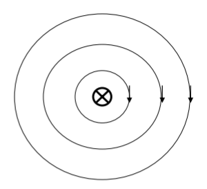
One example of a solenoidal field is a static magnetic field. The field lines do not emanate from or converge to any point, and thus the divergence is zero ( ), and thus
  where A is a vector potential.
2.3 Green’s Identities
In this section, we will discuss about the Divergence theorem and the Green’s first, second, and third identities, which were first published in 1828 by an English mathematician George Green. More information about him can be found in the following links: https://uh.edu/engines/epi1924.htm, https://sites.math.washington.edu/~morrow/334_19/green.pdf, and https://cosmosmagazine.com/mathematics/this- week-in-science-history-england-s-enigmatic- mathematician-is-born
2.3.1 Divergence theorem
Mathematically speaking, the Divergence theorem can be written as the following,
![\begin{equation*} \[\iiint_{V}{\left( \nabla \cdot \mathbf{F} \right)}dV=\mathop{{\int\!\!\!\!\!\int}\mkern-21mu \bigcirc}\nolimits_S \left( \mathbf{F}\cdot \mathbf{n} \right) dS\] \end{equation*}](https://uhlibraries.pressbooks.pub/app/uploads/quicklatex/quicklatex.com-eeed503bdaa7068ea8323cfcaae9edc6_l3.png "Rendered by QuickLaTeX.com")
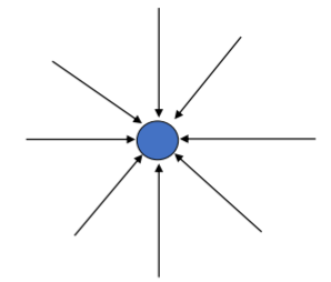
where the left-hand side of this equation represents the volume integral of the divergence over the region inside the surface, while the right-hand side of the equation represents the outward flux of a vector field through a closed surface. The physical meaning can be illustrated through the cartoon image below.
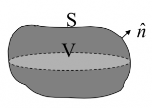
Intuitively, it states that the sum of all sources (with sinks regarded as negative sources) gives the net flux out of a region.
2.3.1.1 Application to gravity
Now, if we consider the vector field as the gravity field  , so that
  , then let’s substitute it into the above divergence theorem equation, we’ll get the following:
![\begin{equation*} \[\iiint\limits_{V}{\left( \nabla \cdot \mathbf{g} \right)}dV=\iint\limits_{S}{\left( \mathbf{g}\cdot \mathbf{\hat{n}} \right)}dS\] \end{equation*}](https://uhlibraries.pressbooks.pub/app/uploads/quicklatex/quicklatex.com-239c0ea8cf4eee9aaef6ac87d7d30270_l3.png "Rendered by QuickLaTeX.com")
From the previous section, we know that  , therefore, replacing , we will get the equation as follows:
![\begin{equation*} \[\begin{align} & \iiint\limits_{V}{\left( \nabla \cdot \nabla \phi \right)}dV=\iint\limits_{S}{\left( \mathbf{g}\cdot \mathbf{\hat{n}} \right)}dS \\ & i.e.,\text{ }\iiint\limits_{V}{\left( {{\nabla }^{2}}\phi \right)}dV=\iint\limits_{S}{\left( \mathbf{g}\cdot \mathbf{\hat{n}} \right)}dS \\ \end{align}\] \end{equation*}](https://uhlibraries.pressbooks.pub/app/uploads/quicklatex/quicklatex.com-da7b177a772774d2379c70a6423b9d89_l3.png "Rendered by QuickLaTeX.com")
Remembering that
![\begin{equation*} \[{{\nabla }^{2}}\phi =-4\pi \gamma \rho \] \end{equation*}](https://uhlibraries.pressbooks.pub/app/uploads/quicklatex/quicklatex.com-79b8c6a74228fec7b52b45cca03c4f37_l3.png "Rendered by QuickLaTeX.com")
therefore, the above equation can be re-arranged into the format below:
![\begin{equation*} \[-4\pi \gamma \iiint\limits_{V}{\rho }dV=\iint\limits_{S}{\left( \mathbf{g}\cdot \mathbf{\hat{n}} \right)}dS\] \end{equation*}](https://uhlibraries.pressbooks.pub/app/uploads/quicklatex/quicklatex.com-92f093855337702cd6e8524b7e315dc8_l3.png "Rendered by QuickLaTeX.com")
It can be noticed that the left-hand side integration gives the quantity of mass,  , thus, the above equation can be further simplified as follows:
![\begin{equation*} \[\begin{align} & -4\pi \gamma M=\iint\limits_{S}{\left( \mathbf{g}\cdot \mathbf{\hat{n}} \right)}dS \\ & \because \text{ }M=-\frac{1}{4\pi \gamma }\iint\limits_{S}{\left( \mathbf{g}\cdot \mathbf{\hat{n}} \right)}dS \\ \end{align}\] \end{equation*}](https://uhlibraries.pressbooks.pub/app/uploads/quicklatex/quicklatex.com-b6bffaeb5cc3ec54c05cc39d097d9ada_l3.png "Rendered by QuickLaTeX.com")
where the right-hand side of this equation contains the surface integral of the flux of the gravity field through a closed surface.
This equation implies that, if we do an integration of the gravity map over a study area, the integration gives an estimate of the mass underneath the gravity map, that is responsible for the measured gravity data.
Before moving to the Green’s identities, let’s review two equations that will be used later.
![\[\nabla }^{2}}\left( \frac{1}{r} \right)=-4\pi \delta \left( r \right)=0,\text{ if }r\ne 0\]](https://uhlibraries.pressbooks.pub/app/uploads/quicklatex/quicklatex.com-007d206c6dc01d8192277a43e6aadb8f_l3.png "Rendered by QuickLaTeX.com")
and
![\[{{\nabla }^{2}}V=-4\pi \gamma \rho\]](https://uhlibraries.pressbooks.pub/app/uploads/quicklatex/quicklatex.com-bfba9db6843a3e4a9fdfda47a2b5d165_l3.png "Rendered by QuickLaTeX.com")
2.3.2 Green’s identities
The three identities can be derived from the vector calculus and the Laplace’s equation. Each of the three identities has different utility and implications for potential field study, and their common starting point is the divergence theorem (aka., Gauss’s theorem) discussed above.
2.3.2.1 Green’s first identity
Let’s assume that there are
- two continuous functions
 with continuous first-order partial derivative;
 - and
 also second-order derivative that’s also continuous;
 - Then defining an arbitrary vector

Applying the divergence theorem, i.e., replacing vector field with  , we will have the following equation:
![\begin{equation*} \[\iiint\limits_{Vol}{\nabla \cdot \left( V\nabla U \right)}dV=\iint\limits_{Surf}{V\nabla U\cdot \mathbf{\hat{n}}}dS\] \end{equation*}](https://uhlibraries.pressbooks.pub/app/uploads/quicklatex/quicklatex.com-a7a48095a29800d9c0205243a874c022_l3.png "Rendered by QuickLaTeX.com")
Then, let’s use the vector identity
![\begin{equation*} \[\nabla \cdot \left( \alpha \mathbf{V} \right)=\alpha \nabla \cdot \mathbf{V}+\nabla \alpha \cdot \mathbf{V}\] \end{equation*}](https://uhlibraries.pressbooks.pub/app/uploads/quicklatex/quicklatex.com-a906061b60f8f09717dbf37451c8848c_l3.png "Rendered by QuickLaTeX.com")
to expand the above divergence theorem equation, we will then get the Green’s first identity as follows:
Green’s first identity
![\begin{equation*} \[\iiint\limits_{Vol}{\left( V{{\nabla }^{2}}U+\nabla V\cdot \nabla U \right)}dV=\iint\limits_{Surf}{V\frac{\partial U}{\partial \mathbf{\hat{n}}}}dS\] \end{equation*}](https://uhlibraries.pressbooks.pub/app/uploads/quicklatex/quicklatex.com-4efeea46c82b02cec78c0cfad6dfd181_l3.png "Rendered by QuickLaTeX.com")
Implication for gravity – 1
If making some simplifications by setting  , and choose U such that
  that satisfies the Laplacian equation (i.e., U is harmonic and its second-order derivative is continuous), then, based on Green’s first identity written above, we will have the following expression
![\begin{equation*} \[\iint\limits_{S}{\frac{\partial U}{\partial \mathbf{\hat{n}}}}dS=0\] \end{equation*}](https://uhlibraries.pressbooks.pub/app/uploads/quicklatex/quicklatex.com-be759b475cd50f8f74afb79e7cf6b9cb_l3.png "Rendered by QuickLaTeX.com")
which can be interpreted as, the normal derivative of a harmonic function averages to 0 on a closed surface.
Specifically for the case of gravity, considering a gravity field in regions of space not occupied by mass, it is associated with a potential which is harmonic. Thus, the above equation can be written as follows:
![\begin{equation*} \[\iint\limits_{S}{\frac{\partial U}{\partial \mathbf{\hat{n}}}}dS=\iint\limits_{S}{\nabla U\cdot \mathbf{\hat{n}}}dS=\iint\limits_{S}{\mathbf{g}\cdot \mathbf{\hat{n}}}dS=0\] \end{equation*}](https://uhlibraries.pressbooks.pub/app/uploads/quicklatex/quicklatex.com-ce37a310be6763fd83a795c5a5020d38_l3.png "Rendered by QuickLaTeX.com")
That is, the gravity field has a net zero flux over any closed surface in any source-free regions (i.e., regions not occupied by sources). This interpretation can be illustrated by the image below.
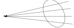
In other words, the normal component of gravity field (or, in general, any conservative field) averages to zero over any closed surface in source-free regions.
Implication for gravity – 2
Another interesting consequence of applying Green’s first identity to potential field is that, if letting be harmonic and  , then we will have
![\begin{equation*} \[{{\iiint\limits_{Vol}{\left( \nabla U \right)}}^{2}}dV=\iint\limits_{Surf}{U\frac{\partial U}{\partial \mathbf{\hat{n}}}}dS\] \end{equation*}](https://uhlibraries.pressbooks.pub/app/uploads/quicklatex/quicklatex.com-4b75fa98f252c69376ba20770ba8bc85_l3.png "Rendered by QuickLaTeX.com")
Consider the above equation when  on the surface
  . Then the R.H.S vanishes, and because
  is positive and continuous in the region, then
  . Therefore, is constant. Moreover, because on the surface and is continuous, the constatn must be 0. Therefore, if is harmonic and continuously differentiable in
  , and if vanishes everywhere on the surface , must also vanish everywhere within the volume.
Furthermore, let  and
and  be harmonic in R and have identical boundary conditions, that is,
  . The function
  must be harmonic. But
  vanishes on S. Based on previous consequence, must vanish at every point in R. Therefore, and are identical. Thus, a function that is harmonic and continuously differentiable in R is uniquely determined by its values on S.
2.3.2.2 Green’s second identity
Based on the assumption that functions and  are continuous functions with continuous second-order derivatives, we can start from the Green’s first identity
then exchange function with to get the function as follows:
![\begin{equation*} \[\iiint\limits_{Vol}{\left( U{{\nabla }^{2}}V+\nabla U\cdot \nabla V \right)}dV=\iint\limits_{Surf}{U\frac{\partial V}{\partial \mathbf{\hat{n}}}}dS\] \end{equation*}](https://uhlibraries.pressbooks.pub/app/uploads/quicklatex/quicklatex.com-3866f8b416867008d521c1dfa6656535_l3.png "Rendered by QuickLaTeX.com")
If subtracting the above equation from the original first identity, we will get the Green’s second identity defined as follows:
![\begin{equation*} \[\iiint\limits_{Vol}{\left( V{{\nabla }^{2}}U-U{{\nabla }^{2}}V \right)}dV=\iint\limits_{Surf}{\left( V\frac{\partial U}{\partial \mathbf{\hat{n}}}-U\frac{\partial V}{\partial \mathbf{\hat{n}}} \right)}dS\] \end{equation*}](https://uhlibraries.pressbooks.pub/app/uploads/quicklatex/quicklatex.com-b9c3bb58dc71adf02d676cdd4b59dc23_l3.png "Rendered by QuickLaTeX.com")
That is,
Green’s second identity
![\begin{equation*} \[\iiint\limits_{Vol}{\left( V{{\nabla }^{2}}U-U{{\nabla }^{2}}V \right)}dV=\iint\limits_{Surf}{\left( V\nabla U-U\nabla V \right)\cdot \mathbf{\hat{n}}}dS\] \end{equation*}](https://uhlibraries.pressbooks.pub/app/uploads/quicklatex/quicklatex.com-aa2cea00cc527f2735d4befaebece0a5_l3.png "Rendered by QuickLaTeX.com")
Implication for gravity – 1
So how can this identity be related with potential field methods? If assuming , then the Green’s second identity can be re-written as follows:
![\begin{equation*} \[\iiint\limits_{Vol}{{{\nabla }^{2}}U}dV=\iint\limits_{Surf}{\nabla U\cdot \mathbf{\hat{n}}}dS\] \end{equation*}](https://uhlibraries.pressbooks.pub/app/uploads/quicklatex/quicklatex.com-21f9339107cb5d9920157cc8a534eea5_l3.png "Rendered by QuickLaTeX.com")
and assuming is the potential of some vector field , i.e.,  , then the above equation can be further written as:
![\begin{equation*} \[\iiint\limits_{Vol}{{{\nabla }^{2}}U}dV=\iint\limits_{Surf}{\mathbf{F}\cdot \mathbf{\hat{n}}}dS\] \end{equation*}](https://uhlibraries.pressbooks.pub/app/uploads/quicklatex/quicklatex.com-6a3b1a108641dea43d38e389f7753410_l3.png "Rendered by QuickLaTeX.com")
In source-free regions, , therefore, we have
![\begin{equation*} \[0=\iint\limits_{Surf}{\mathbf{F}\cdot \mathbf{\hat{n}}}dS\] \end{equation*}](https://uhlibraries.pressbooks.pub/app/uploads/quicklatex/quicklatex.com-eb60df42bb7898867be1aafd8528ec2f_l3.png "Rendered by QuickLaTeX.com")
which implies that, the net flux of gravitational field over a surface with source-free equals zero, the same conclusion we derived before.
Implication for gravity – 2
In Green’s second identity, the surface is a closed surface bounding the volume. For gravity application, it is a surface bounding the mass. Now let’s consider a special surface: an equipotential surface. Assuming function as gravity potential, and consider a point outside the surface, and is the distance from . Let’s consider what happens when  .
.
We can substitute into the second identity, then we will have the following:
![\begin{equation*} \[\iiint\limits_{Vol}{\left( V{{\nabla }^{2}}\left( \frac{1}{r} \right)-\frac{1}{r}{{\nabla }^{2}}V \right)}dV=\iint\limits_{Surf}{\left( V\nabla \left( \frac{1}{r} \right)-\frac{1}{r}\nabla V \right)\cdot \mathbf{\hat{n}}}dS\] \end{equation*}](https://uhlibraries.pressbooks.pub/app/uploads/quicklatex/quicklatex.com-e815066d3f4f91eb0dcf8a18d4fdc1c9_l3.png "Rendered by QuickLaTeX.com")
Recall the two equations defined above, which are  and
and  , then the above equation’s left-hand side can be simplied as follows:
![\begin{equation*} \[\iiint\limits_{Vol}{\left( V{{\nabla }^{2}}\left( \frac{1}{r} \right)-\frac{1}{r}{{\nabla }^{2}}V \right)}dV=4\pi \gamma \iiint\limits_{Vol}{\frac{\rho }{r}}dV\] \end{equation*}](https://uhlibraries.pressbooks.pub/app/uploads/quicklatex/quicklatex.com-6a0249a9f532f9e7756d110b4aa88f63_l3.png "Rendered by QuickLaTeX.com")
For the right-hand side, since gravity potential is constant on the equipotential surface, so can be moved out of the integral; then we can apply the divergence theorem, so that the surface integral can be changed to colume integral. Their mathematical expressions are as follows:
![\begin{equation*} \[\begin{align} & \iint\limits_{Surf}{V\nabla \left( \frac{1}{r} \right)\cdot \mathbf{\hat{n}}}dS=V\iint\limits_{Surf}{\nabla \left( \frac{1}{r} \right)\cdot \mathbf{\hat{n}}}dS \\ & \iint\limits_{Surf}{\nabla \left( \frac{1}{r} \right)\cdot \mathbf{\hat{n}}}dS=\iiint\limits_{Vol}{{{\nabla }^{2}}\left( \frac{1}{r} \right)}dV \\ \end{align}\] \end{equation*}](https://uhlibraries.pressbooks.pub/app/uploads/quicklatex/quicklatex.com-7123dd8bda2b8e664ce31e74ae30d192_l3.png "Rendered by QuickLaTeX.com")
Now, recall the Laplacian of inverse distance
![\begin{equation*} \[\iint\limits_{Surf}{V\nabla \left( \frac{1}{r} \right)\cdot \mathbf{\hat{n}}}dS=0\] \end{equation*}](https://uhlibraries.pressbooks.pub/app/uploads/quicklatex/quicklatex.com-ae845aba52468a743143401e7251cf3a_l3.png "Rendered by QuickLaTeX.com")
Thus, the second identity can be written as follows:
![\begin{equation*} \[4\pi \gamma \iiint\limits_{Vol}{\frac{\rho }{r}}dV=-\iint\limits_{Surf}{\frac{1}{r}\nabla V\cdot \mathbf{\hat{n}}}dS\] \end{equation*}](https://uhlibraries.pressbooks.pub/app/uploads/quicklatex/quicklatex.com-74e1b81b25942cbc5899b78901aa9683_l3.png "Rendered by QuickLaTeX.com")
If we look carefully on the left-hand side of the above equation, it contains the calculation of the gravitational potenital given a density distributino, which equals  , therefore, we have,
![\begin{equation*} \[4\pi {{V}_{p}}=4\pi \gamma \iiint\limits_{Vol}{\frac{\rho }{r}}dV=-\iint\limits_{Surf}{\frac{1}{r}\nabla V\cdot \mathbf{\hat{n}}}dS\] \end{equation*}](https://uhlibraries.pressbooks.pub/app/uploads/quicklatex/quicklatex.com-f4786f989719e6466036364af2082c8e_l3.png "Rendered by QuickLaTeX.com")
dividing  on both sides, we will have
![\begin{equation*} \[{{V}_{p}}=\gamma \iiint\limits_{Vol}{\frac{\rho }{r}}dV=-\frac{1}{4\pi }\iint\limits_{Surf}{\frac{1}{r}\nabla V\cdot \mathbf{\hat{n}}}dS\] \end{equation*}](https://uhlibraries.pressbooks.pub/app/uploads/quicklatex/quicklatex.com-9c63f27ee840f8720b1f68e42c84df21_l3.png "Rendered by QuickLaTeX.com")
This equation implies that for a set of gravitational field data, it can be interpreted by two methods: at any point outside , the potential caused by a 3d source inside is the same as the potential caused by a material that is spread over the equipotential surface with a surface density of  .
.
2.3.2.3 Green’s third identity
Its derivation begins with second identity
Again, let’s make simplifications by letting where the second identity will then be written as follows
![\begin{equation*} \[\iiint\limits_{Vol}{\left( V{{\nabla }^{2}}\frac{1}{r}-\frac{1}{r}{{\nabla }^{2}}V \right)}dV=\iint\limits_{Surf}{\left( V\nabla \frac{1}{r}-\frac{1}{r}\nabla V \right)\cdot \mathbf{\hat{n}}dS}\] \end{equation*}](https://uhlibraries.pressbooks.pub/app/uploads/quicklatex/quicklatex.com-74dd2e16fa6d6241f33caae98cded4c0_l3.png "Rendered by QuickLaTeX.com")
Remembering that  in general case (i.e., can be zero within the volume). Then the above equation can be re-written as follows:
![\begin{equation*} \[\iiint\limits_{Vol}{\left( -4\pi V\delta \left( r \right)-\frac{1}{r}{{\nabla }^{2}}V \right)}dV=\iint\limits_{Surf}{\left( V\nabla \frac{1}{r}-\frac{1}{r}\nabla V \right)}\cdot \mathbf{\hat{n}}dS\] \end{equation*}](https://uhlibraries.pressbooks.pub/app/uploads/quicklatex/quicklatex.com-6f179e64d345b89e4a0fe315a89374ff_l3.png "Rendered by QuickLaTeX.com")
Moving the second term on the left to the R.H.S., we have
![\begin{equation*} \[\iiint\limits_{Vol}{-4\pi V\delta \left( r \right)}dV=\iiint\limits_{Vol}{\frac{1}{r}{{\nabla }^{2}}VdV+}\iint\limits_{Surf}{\left( V\nabla \frac{1}{r}-\frac{1}{r}\nabla V \right)}\cdot \mathbf{\hat{n}}dS\] \end{equation*}](https://uhlibraries.pressbooks.pub/app/uploads/quicklatex/quicklatex.com-0839140f8bf5e5d89cf6708f36b5cb1d_l3.png "Rendered by QuickLaTeX.com")
Diving by  on both sides, and expand further, the new equation will be
![\begin{equation*} \[\iiint\limits_{Vol}{V\delta \left( r \right)}dV=-\frac{1}{4\pi }\iiint\limits_{Vol}{\frac{1}{r}{{\nabla }^{2}}VdV-}\frac{1}{4\pi }\iint\limits_{Surf}{V\nabla \frac{1}{r}}\cdot \mathbf{\hat{n}}dS+\frac{1}{4\pi }\iint\limits_{Surf}{\frac{1}{r}\nabla V}\cdot \mathbf{\hat{n}}dS\] \end{equation*}](https://uhlibraries.pressbooks.pub/app/uploads/quicklatex/quicklatex.com-7b48ff377cb2f9077e0b0740e16ebce5_l3.png "Rendered by QuickLaTeX.com")
Based on the definition of derivatives, the R.H.S. of the previous equation can be re-written as
![\begin{equation*} \[\iiint\limits_{Vol}{V\delta \left( r \right)}dV=-\frac{1}{4\pi }\iiint\limits_{Vol}{\frac{1}{r}{{\nabla }^{2}}VdV-}\frac{1}{4\pi }\iint\limits_{Surf}{V\frac{\partial }{\partial \mathbf{\hat{n}}}\frac{1}{r}}dS+\frac{1}{4\pi }\iint\limits_{Surf}{\frac{1}{r}\frac{\partial V}{\partial \mathbf{\hat{n}}}}dS\] \end{equation*}](https://uhlibraries.pressbooks.pub/app/uploads/quicklatex/quicklatex.com-718787ca94a9bad0d78dad05552c4217_l3.png "Rendered by QuickLaTeX.com")
According to the definition of the Dirac delta function,
![\begin{equation*} \[\begin{align} & \delta \left( x \right)=\left\{ \begin{matrix} +\infty ,\text{ }x=0 \\ 0,\text{ }x\ne 0 \\ \end{matrix} \right. \\ & \int_{-\infty }^{\infty }{\delta \left( x \right)dx=1} \\ & \int_{-\infty }^{\infty }{f\left( x \right)\delta \left( x \right)dx=f\left( 0 \right)} \\ \end{align}\] \end{equation*}](https://uhlibraries.pressbooks.pub/app/uploads/quicklatex/quicklatex.com-7b3787db35a23683655984d06b76a069_l3.png "Rendered by QuickLaTeX.com")
Through applying the Dirac delta function property, the above equation will be the Green’s third identity. For simplicity, we assumed the origin to be the point of observation, therefore, we will have:
![\begin{equation*} \[V\left( 0 \right)=-\frac{1}{4\pi }\iiint\limits_{Vol}{\frac{1}{r}{{\nabla }^{2}}VdV-}\frac{1}{4\pi }\iint\limits_{Surf}{V\frac{\partial }{\partial \mathbf{\hat{n}}}\frac{1}{r}}dS+\frac{1}{4\pi }\iint\limits_{Surf}{\frac{1}{r}\frac{\partial V}{\partial \mathbf{\hat{n}}}}dS\] \end{equation*}](https://uhlibraries.pressbooks.pub/app/uploads/quicklatex/quicklatex.com-6d9b0fabf3327880c2485da57a0fed32_l3.png "Rendered by QuickLaTeX.com")
In general, for a continuous function , the Green’s third identity is
Green’s third identity
![\begin{equation*} \[V\left( P \right)=-\frac{1}{4\pi }\iiint\limits_{Vol}{\frac{1}{r}{{\nabla }^{2}}VdV-}\frac{1}{4\pi }\iint\limits_{Surf}{V\frac{\partial }{\partial \mathbf{\hat{n}}}\frac{1}{r}}dS+\frac{1}{4\pi }\iint\limits_{Surf}{\frac{1}{r}\frac{\partial V}{\partial \mathbf{\hat{n}}}}dS\] \end{equation*}](https://uhlibraries.pressbooks.pub/app/uploads/quicklatex/quicklatex.com-2e4d059e5e2819c6ddca4feebf9775e4_l3.png "Rendered by QuickLaTeX.com")
Understanding Green’s third identity
The first integral on the R.H.S. of the Green’s third identity can be understood as the potential due to a volume distribution with density  , that is, the gravitational potential due to a volume density distribution
  is
is
![\begin{equation*} \[V\left( P \right)=\gamma \iiint\limits_{Vol}{\frac{\rho \left( Q \right)}{r}dV}\] \end{equation*}](https://uhlibraries.pressbooks.pub/app/uploads/quicklatex/quicklatex.com-02a018ef299874c639dab2be0316f766_l3.png "Rendered by QuickLaTeX.com")
The third integral has the same form as the potential due to a surface density distribution  where
where  . That is, the gravitational potential due to a surface density distribution
  is
is
![\begin{equation*} \[V\left( P \right)=\gamma \iint\limits_{Surf}{\frac{\sigma \left( Q \right)}{r}}dS\] \end{equation*}](https://uhlibraries.pressbooks.pub/app/uploads/quicklatex/quicklatex.com-a353f923dc639778a0dee26463008d21_l3.png "Rendered by QuickLaTeX.com")
The second integral can be understood as the magmatic potential due to a surface distribution of magnetization  , which is spread over surface , and directed normal to . The magnetic potential is
![\begin{equation*} \[V\left( P \right)=\frac{{{\mu }_{0}}}{4\pi }\iint\limits_{Surf}{\mathbf{M}\left( Q \right)\mathbf{\hat{n}}\cdot {{\nabla }_{Q}}\frac{1}{r}}dS=\frac{{{\mu }_{0}}}{4\pi }\iint\limits_{Surf}{\mathbf{M}\left( Q \right)\frac{\partial }{\partial \mathbf{\hat{n}}}\frac{1}{r}}dS\] \end{equation*}](https://uhlibraries.pressbooks.pub/app/uploads/quicklatex/quicklatex.com-3b845469bcdfc7805f3b6903785cc028_l3.png "Rendered by QuickLaTeX.com")
In summary, any function with sufficient differentiability can be expressed as the sum of three potentials:
- The potential due to a volume distribution of density
- The potential due to a surface distribution of density

- The potential due to a surface distribution of magnetization
In other words, any function with sufficient differentiability is a potential!
Furthermore, if considering the situation when is harmonic, i.e., , then Green’s third identity will become the following
![\begin{equation*} \[\begin{align} & V\left( P \right)=-\frac{1}{4\pi }\iint\limits_{Surf}{V\frac{\partial }{\partial \mathbf{\hat{n}}}\frac{1}{r}}dS+\frac{1}{4\pi }\iint\limits_{Surf}{\frac{1}{r}\frac{\partial V}{\partial \mathbf{\hat{n}}}}dS \\ & i.e.,\text{ }V\left( P \right)=\frac{1}{4\pi }\iint\limits_{Surf}{\left( \frac{1}{r}\frac{\partial V}{\partial \mathbf{\hat{n}}}-V\frac{\partial }{\partial \mathbf{\hat{n}}}\frac{1}{r} \right)}dS \\ \end{align}\] \end{equation*}](https://uhlibraries.pressbooks.pub/app/uploads/quicklatex/quicklatex.com-beab0cb3404c329b14da8085ae2d9155_l3.png "Rendered by QuickLaTeX.com")
This is a representation formula, where a harmonic function can be calculated at any point simply from its values and normal derivatives on the boundary. This is the theoretical basis for the upward continuation and the equivalent source technique, which will be introduced later in this course.
2.4 Gravitational Potential
2.4.1 Newtonian Potential
There are four basic forces known presently to physics, which are strong force, electromagnetic force, weak force, and gravitational force.
- Strong force could hold protons and neutrons together in the atomic nucleus and have extremely short range, but a hundred times more powerful than electrical forces.
- Electromagnetic force, for instance, the electrostatic force following the Coulomb’s law, could produce the everyday phenomenon of static electricity, or lightning strike due to sudden electrostatic discharge. Another exampl
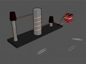 e is the magnetic force, generated by a magnet. In a simple experiment setting shown in the figure on the right, if the coil wired around the metal is powered with electricity, that will generate a magnetic field, which will then make this metal becomes serving as a magnet.
 - Weak force accounts for certain kinds of radioactive decay.
- Gravitational force, which is the force that we will focus on in this course. Unfortunately, we do not fully understand gravity, despite Newton’s law of gravitational attraction and Einstein’s general relativity.
In this course, we will focus on Newton’s law of gravitational attraction to discuss the gravitational force.
2.4.1.1 Gravity attraction
Issac Newton was an English mathematician, physicist, astronomer, theologian and author who lived in the time period of 1642-1726. He had made fundamental contributions to classical mechanics, optics and calculus, and published the famous Mathematical Principle of Natural Philosophy in 1687. In this book, Newton formulated the laws of motion and the law of gravitational attraction.
Newton’s law of gravitational attraction
The simple illustration of Newton’s law of gravitational attraction is shown in the figure below.
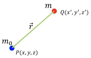
The mutual force between the two masses and  is mathematically represented as:
![\[F=\gamma \frac{m{{m}_{0}}}{{{r}^{2}}}\]](https://uhlibraries.pressbooks.pub/app/uploads/quicklatex/quicklatex.com-0978d53e992bcd56fdfbbaaa7ab3481c_l3.png "Rendered by QuickLaTeX.com")
![\[r=\sqrt{{{\left( x-{x}' \right)}^{2}}+{{\left( y-{y}' \right)}^{2}}+{{\left( z-{z}' \right)}^{2}}}\]](https://uhlibraries.pressbooks.pub/app/uploads/quicklatex/quicklatex.com-e45c023e3f20c81f2b7427801ffb8c4f_l3.png "Rendered by QuickLaTeX.com")
where is the distance between two masses,  is the universal gravitational constant.
Let us consider to be a test particle with unit mass (i.e., the existence of it doesn’t affect the force caused by mass ). Then the gravitational attraction produced by mass at the location of the test particle is
![\[\vec{g}\left( P \right)=-\gamma \frac{m}{{{r}^{2}}}\mathbf{\hat{r}}\]](https://uhlibraries.pressbooks.pub/app/uploads/quicklatex/quicklatex.com-af73ea28393f9d313924d217cf2b57c4_l3.png "Rendered by QuickLaTeX.com")
Note is gone since we have assumed it is a test particle with unit mass, and the unit vector is pointing from to . The minus sign in this equation is necessary because  , following convention, is directly from the source to the observation point .
The unit of this gravitational attraction  can be derived from the following:
![\[\mathbf{g}(P)=\frac{F}{{{m}_{0}}}=\frac{\gamma \frac{m{{m}_{0}}}{{{r}^{2}}}}{{{m}_{0}}}=\gamma \frac{m}{{{r}^{2}}}\]](https://uhlibraries.pressbooks.pub/app/uploads/quicklatex/quicklatex.com-8aaf916dafa0e3296381f368c2caf62c_l3.png "Rendered by QuickLaTeX.com")
i.e., is force divided by mass, therefore it has the unit of acceleration,  .
.
Therefore, the gravitational attraction is also called gravitational acceleration, and it is a vector since the gravitational force has a direction. Its values vary depending on the measured locations on Earth, its conventional standard value is about 9.8 m/s2.
After-class Exercises
Given 
Prove 
*Hint: it is easier to do the proof in spherical coordinate.
Once we have proved ourselves after doing the exercise listed on the right box, that
![\[\nabla \times \mathbf{g}=0\]](https://uhlibraries.pressbooks.pub/app/uploads/quicklatex/quicklatex.com-7d3405ebd7cd8160fe616990fc24ef2f_l3.png "Rendered by QuickLaTeX.com")
we can interpret and make sense of it since, for Earth, its gravitational field lines are all pointing to its center from 360o degrees, thus there is no rotation, so the curl must be zero.
That brings us to the concept of the irrotational field when we talked about the Helmholtz theorem. An irrotational field is a vector field in a region if its curl vanishes everywhere, i.e.,
![\[\nabla \times \mathbf{F}=0\]](https://uhlibraries.pressbooks.pub/app/uploads/quicklatex/quicklatex.com-5c1deb55157d61cf6dcad2e0ac05af3e_l3.png "Rendered by QuickLaTeX.com")
that is, when the curl of a vector field is zero, the field is irrotational. Since the gravitational field satisfies this condition, therefore, the gravitational field is irrotational.
Moreover, according to the Helmholtz theorem, the vector potential becomes zero. Therefore,
![\[\mathbf{F}=\nabla \phi\]](https://uhlibraries.pressbooks.pub/app/uploads/quicklatex/quicklatex.com-b245fc3fb0a087ab72038a7773e24ce1_l3.png "Rendered by QuickLaTeX.com")
which is a scalar potential, or gravitational potential.
In brief summary, because , the Gravitational/Newtonian potential is irrotational and is conservative. It can be fully described by a scalar potential  , where is called gravitational potential, and it can be mathematically represented as follows:
![\[U=\gamma \frac{m}{r}\]](https://uhlibraries.pressbooks.pub/app/uploads/quicklatex/quicklatex.com-cde6341e887d34ae58b623519cc7dac1_l3.png "Rendered by QuickLaTeX.com")
which decays as a function of distance .
2.4.1.2 Gravitational potential of continuous matter
For the sake of convenience and robustness, we want to be able to calculate the gravitational potential due to any distribution of density with any geometries. Thus, we need to apply the Principle of Superposition, so that the gravitational potential of a collection of masses can be calculated as a sum of the gravitational potentials due to each individual mass.
Similarly, the gravitational field/acceleration, which is a vector, of a collection of masses is the vector sum of the gravitational acceleration due to each individual mass.
If we want to calculate the gravitational attraction due to a continuous distribution of matter, that is density  varies spatially, we can use the principle of superposition, so that the continuous distribution of mass is simply a collection of many very small masses. For each small mass, its individual mass can be calculated by the product of constant density of this small mass with its volume occupied by the tiny mass
  , that is,
![\[dm = \rho (x, y, z) dv\]](https://uhlibraries.pressbooks.pub/app/uploads/quicklatex/quicklatex.com-dfab1eeb130c0f3ab3f504b7503d10d4_l3.png "Rendered by QuickLaTeX.com")
The gravitational potential due to this single small mass is
![\[U(P)=\gamma \frac{dm}{r}\]](https://uhlibraries.pressbooks.pub/app/uploads/quicklatex/quicklatex.com-efd9e2f9427554fcf208b0f1c90a8f0d_l3.png "Rendered by QuickLaTeX.com")
Then the potential observed at location due to all small masses can be then calculated by summation of all individual potentials, i.e., the integration over the whole volume occupied by mass at each point of  within the volume, which is mathematically written as follows:
![\[U(P)=\gamma \int\limits_{v}{\frac{dm}{r}=}\gamma \int\limits_{v}{\frac{\rho (Q)dv}{r}}\]](https://uhlibraries.pressbooks.pub/app/uploads/quicklatex/quicklatex.com-0c2f3415ff3a79c03c01025e1b02d786_l3.png "Rendered by QuickLaTeX.com")
According to Helmholtz theorem, we know that  . Thus, in order to calculate gravity, we need to calculate
![\[\frac{\partial U(P)}{\partial x}=\gamma \frac{\partial }{\partial x}\int\limits_{v}{\frac{\rho (Q)dv}{r}}=\gamma \int\limits_{v}{\frac{\partial }{\partial x}}\frac{1}{r}\rho (Q)dv=-\gamma \int\limits_{v}{\frac{x-{x}'}{{{r}^{3}}}\rho (Q)dv}\]](https://uhlibraries.pressbooks.pub/app/uploads/quicklatex/quicklatex.com-f66f91744c2fe81e9ac690aef500d7f0_l3.png "Rendered by QuickLaTeX.com")
Similarly, following the same procedure, we can calculate  , i.e.,
![\begin{equation*} \[\begin{align} & \frac{\partial U(P)}{\partial x}= -\gamma \int\limits_{v}{\frac{x-{x}'}{{{r}^{3}}}\rho (Q)dv}\\ & \frac{\partial U(P)}{\partial y} = -\gamma \int\limits_{v}{\frac{y-{y}'}{{{r}^{3}}}\rho (Q)dv}\\ & \frac{\partial U(P)}{\partial z} = -\gamma \int\limits_{v}{\frac{z-{z}'}{{{r}^{3}}}\rho (Q)dv}\\ \end{align}\] \end{equation*}](https://uhlibraries.pressbooks.pub/app/uploads/quicklatex/quicklatex.com-d90f451845011e7daf425ce37dc31483_l3.png "Rendered by QuickLaTeX.com")
If we collect the three terms on the left hand side in the above three equations into a vector, we get  which is equal to . The three integrals on the right hand side in the above three equations can also be collapsed into a more compact form. Consequently, we arrive at the following equation:
![\begin{equation*} \[\begin{align} & \mathbf{g}(P)=-\gamma \int\limits_{V}{\rho (Q)\frac{{\vec{r}}}{{{r}^{3}}}}dv\\ & i.e., \mathbf{g}(P)=-\gamma \int\limits_{V}{\rho (Q)\frac{{\hat{r}}}{{{r}^{2}}}}dv\\ \end{align}\] \end{equation*}](https://uhlibraries.pressbooks.pub/app/uploads/quicklatex/quicklatex.com-0342e64560f44b24ef1f975a91417d61_l3.png "Rendered by QuickLaTeX.com")
where  is the unit vector in the same direction as the vector .
Please be noted that the previous derivation of the gravity field based on gravitational potential assumes the observation point is outside the distribution of mass. What about the potential inside the mass?
If the observation point is inside the mass, the integrand in equation becomes singular and the integral is improper (see P47 in Blakely’s book). However, Kellogg (1953) shows that the integral
![\begin{equation*} \[\begin{align} I(P)= \int\limits_{V}\frac{\rho}{r^n}dv \end{align}\] \end{equation*}](https://uhlibraries.pressbooks.pub/app/uploads/quicklatex/quicklatex.com-cd4b76f6548b830668cd48c431accdb7_l3.png "Rendered by QuickLaTeX.com")
is convergent for inside a volume and is continuous throughout if  , is bounded and is piecewise continuous. Therefore, both
  and exist and are continuous everywhere, both inside and outside the mass if the density in the volume is well behaved (Blakely, 1996, p48). In addition, Kellogg (1957) also shows that for inside the mass.
In summary, the following two equations hold true for any bounded distribution of piecewise-continuous density:
![\begin{equation*} \[\begin{align} \mathbf{g}(P)=-\gamma \int\limits_{V}{\rho (Q)\frac{{\hat{r}}}{{{r}^{2}}}}dv\\ \end{align}\] \end{equation*}](https://uhlibraries.pressbooks.pub/app/uploads/quicklatex/quicklatex.com-c2049c54071d5b14ac7734018d5a5e39_l3.png "Rendered by QuickLaTeX.com")
and
![\begin{equation*} \[\begin{align} $\bm{g}(P) = \nabla U(P)$. \end{align}\] \end{equation*}](https://uhlibraries.pressbooks.pub/app/uploads/quicklatex/quicklatex.com-ee543dfe5b27e171b4f37b5aba938a07_l3.png "Rendered by QuickLaTeX.com")
2.4.1.3 Poisson’s equation
So far, we can represent the gravitational potential in two math equations, one is based on Helmholtz theorem, we have mathematically derived at
![\[U(P)=-\frac{1}{4\pi }\int{\frac{\nabla \cdot \mathbf{g}(Q)}{r}dv}\]](https://uhlibraries.pressbooks.pub/app/uploads/quicklatex/quicklatex.com-acdebfe396f8408bbc32d4f529d43a2b_l3.png "Rendered by QuickLaTeX.com")
another equation is due to Newton’s law of gravitational attraction, which is written as
![\[U(P)=\gamma \int\limits_{V}{\frac{\rho (Q)dv}{r}}\]](https://uhlibraries.pressbooks.pub/app/uploads/quicklatex/quicklatex.com-7329584146bdb5d97ede8ca16832f8ca_l3.png "Rendered by QuickLaTeX.com")
By equalling those two equations, we will arrive at the Poisson’s equation, which is expressed as follows:
![\[\nabla \cdot \mathbf{g}=-4\pi \gamma \rho\]](https://uhlibraries.pressbooks.pub/app/uploads/quicklatex/quicklatex.com-527b5d00f96f19bd922dc61321466b73_l3.png "Rendered by QuickLaTeX.com")
This is valid for observation point both inside and outside the mass distribution.
A special case of Poisson’s equation is Laplace’s equation, which is denoted as below:
![\[\nabla \cdot \mathbf{g}=0\]](https://uhlibraries.pressbooks.pub/app/uploads/quicklatex/quicklatex.com-c098b39858529a9a2b34702e145c8c5a_l3.png "Rendered by QuickLaTeX.com")
which is valid in regions of space not occupied by mass. For most of the geophysical potential field data acquisition, we are dealing with this equation, since the data measurement region is at the source-free region, for example, airborne data acquisition, satellite data collection, etc.
Brief Summary
- Gravitational potential:

- Gravitational field/acceleration:

- Poisson’s equation

2.4.2 Examples of Gravity due to Simple Objects
Before delving into the details of deriving the gravitational response due to simple geometric objects, it is important to note that the following derivations are much simplified due to having to deal with the problem in spherical coordinates. Thus, firstly let us recap on the concept of the spherical coordinate system.
2.4.2.1. Spherical Coordinate System
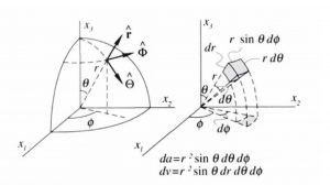
Normally, most problems are done in the Cartesian coordinate system (x, y, z). However, to simplify the integration in our derivation, we use the spherical coordinate system instead. The following figure gives a visualization of the coordinate system. A point in space can be expressed as the point (r,  , ), where r is the distance between the point and the origin, is the declination of the line connecting the point to the origin, and is the inclination (angle made by the line that crosses the origin with the horizontal). With simple trigonometrical calculations, we can find that the small differential area
  can be expressed as
  and the differential volume as
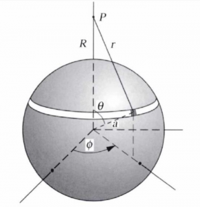
2.4.2.2. Gravity due to Spherical Shell
First, let us consider a thin-walled, spherical shell with radius  and uniform surface density (think about those hollow colorful plastic balls in a kids ball pit, but with much much thinner skin). The ball is perfectly symmetric, and thus we can use this property to form the problem in a spherical coordinate system. We will derive the gravity in point P which is outside of the shell with a distance of R from the shell (r in the figure is the distance of any point in the shell to P).
Recall that the gravitational potential equation from the previous section can be expressed as such:
![\[U(P) = \gamma \int_S \frac{\sigma(Q)}{r} dS\]](https://uhlibraries.pressbooks.pub/app/uploads/quicklatex/quicklatex.com-24e611802bc54594f516516fac9a9bc2_l3.png "Rendered by QuickLaTeX.com")
This is true for a mass distribution that spreads over a vanishingly thin surface, where has a unit of mass per unit area ( in SI).
Transforming the above equation to our spherical coordinate system (that is, substituting  and assuming that
  is constant at the differential area), the above equation can also be expressed as:
![\[U(P) = \gamma \int_0^{2\pi} \int_0^{\pi} \frac{\sigma(Q)}{r} a^2 sin \theta d\theta d\phi = \gamma \sigma a^2 \int_0^{2\pi} \int_0^{\pi} \frac{sin\theta}{r} d\theta d\phi\]](https://uhlibraries.pressbooks.pub/app/uploads/quicklatex/quicklatex.com-98f684bde19fbb44cfe9fb274529b794_l3.png "Rendered by QuickLaTeX.com")
With simple trigonometrical calculations, we can find that 
Since the following relation is true:
![\[\frac{dr}{d\theta} = \frac{aRsin\theta}{r}\]](https://uhlibraries.pressbooks.pub/app/uploads/quicklatex/quicklatex.com-1d05aa42d305553ca775eb55ec9416fb_l3.png "Rendered by QuickLaTeX.com")
![\[sin\theta d\theta / r = dr/aR\]](https://uhlibraries.pressbooks.pub/app/uploads/quicklatex/quicklatex.com-36aa01babf6bdd41ad1e2c71763ecaa6_l3.png "Rendered by QuickLaTeX.com")
That means we can further simplify the equation as:
![\[U(P) = \gamma \sigma a^2 \int_0^{2\pi} \int_0^{\pi} \frac{1}{aR} dr d\phi\]](https://uhlibraries.pressbooks.pub/app/uploads/quicklatex/quicklatex.com-ed44de2def665b07337d49618e90d668_l3.png "Rendered by QuickLaTeX.com")
With that in mind, we can substitute the integral bounds in terms of the radius, with  and
and  being the minimum and the maximum value of respectively, thus turning our gravity potential equation to:
![\[U(P) = \frac{2\pi \gamma \sigma a}{R} \int_{R-a}^{R+a} dr\]](https://uhlibraries.pressbooks.pub/app/uploads/quicklatex/quicklatex.com-88d4f92d00bc8d539f76f940709fd867_l3.png "Rendered by QuickLaTeX.com")
Thus if we evaluate the integral, we can get the gravity potential at point P due to a spherical shell, if P is outside the shell:
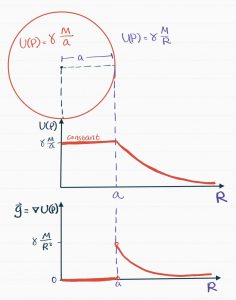
![\[U(P) = \gamma \frac{4\pi a^2 \sigma}{R}\]](https://uhlibraries.pressbooks.pub/app/uploads/quicklatex/quicklatex.com-0071f22aa4264059540f1f7793a43f03_l3.png "Rendered by QuickLaTeX.com")
Since  where M is mass, then the above equation can also be expressed as:
![\[U(P) = \gamma \frac{M}{R}\]](https://uhlibraries.pressbooks.pub/app/uploads/quicklatex/quicklatex.com-cf84cacc2989a4b4d358fb7ed50e6d39_l3.png "Rendered by QuickLaTeX.com")
Notice that this is the same gravity potential from a point source. In other words:
“Gravity potential at any point outside a uniform shell is the same as the potential of a point source located at the center of the shell with mass equal to the total mass of the shell”
We can conclude the same with the gravitational attraction ( ), thus the gravitational attraction at any point outside a uniform shell is the same as the attraction of a point mass. This can be easily verified with
This emphasize the non-uniqueness problem in gravity, since this implies that the same gravity observation can be form by either point source or spherical shell equally well.
Meanwhile, if point P is inside the shell, then the above derivation still holds true but with a small difference in the bounds in the integral, which is:
![\[U(P) = \frac{2\pi \gamma \sigma a}{R} \int_{a-R}^{a+R} dr = \gamma \sigma 4\pi a = \gamma \frac{M}{a}\]](https://uhlibraries.pressbooks.pub/app/uploads/quicklatex/quicklatex.com-fcb1b65def01f8a7f2def8d4c2d842cc_l3.png "Rendered by QuickLaTeX.com")
In this case, the gravitational potential is constant everywhere inside a uniform shell. Thus the gravitational attraction is:
![\[g(P) = \nabla U(P) = \nabla (\gamma \frac{M}{a}) = 0\]](https://uhlibraries.pressbooks.pub/app/uploads/quicklatex/quicklatex.com-498cda2dd1fab11405380bdca2aeee5d_l3.png "Rendered by QuickLaTeX.com")
Thus, the above derivations can be simplified in the following summary:
Gravity due to a uniform spherical shell
- If P is outside the shell, then the following holds true (
 ):
):
- Gravity potential:

- Gravitational attraction:

- Gravity potential:
- If P is inside the shell, then the following holds true:
- Gravity potential:

- Gravitational attraction:

- Gravity potential:
2.4.2.2. Gravity due to a Uniform Solid Sphere
For P outside the sphere, we can consider the sphere as a collection of concentric, thin-walled shells with radii ranging from 0 to a (think of an infinite matryoshka, Russian nested doll, but instead it’s spherical and the skin are much more thin). Thus, we can apply the superposition principle in this case. In other words:
“The potential of a solid sphere at any location outside the sphere is the same as a point mass at the center of the sphere with mass equal to the total mass of the sphere.”
![\[U(P) = \gamma \frac{M}{R} = \gamma \frac{\frac{4}{3}\pi a^3 \rho}{R}\]](https://uhlibraries.pressbooks.pub/app/uploads/quicklatex/quicklatex.com-cf07e2f1b2220aba2aaa776640f5c918_l3.png "Rendered by QuickLaTeX.com")
The derivation in the case of P being inside the sphere requires a bit more understanding.
Suppose that P is in a narrow, spherical cavity of radius r and thickness  indicated in the following figure:
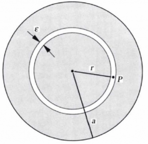
The potential at P is due to two parts:
- The inner part of the sphere with radius less that

- The outer part of the sphere with radius greater than

Let’s first looks at the inner part (first part). Since in the figure above, P is outside of the first part, we can define the gravitational potential as:
![\[U_1 (P) = \gamma \frac{\frac{4}{3}\pi (r-\frac{\epsilon}{2})^3 \rho}{R}\]](https://uhlibraries.pressbooks.pub/app/uploads/quicklatex/quicklatex.com-a1ef5761729ca3a7c2df55ccf53d5297_l3.png "Rendered by QuickLaTeX.com")
Now, for the outer part (second part), the derivation gets more complex, as we can express it as such:
![\[U_2(P) = \gamma \pi \gamma \rho (a^2 - (r + \frac{\epsilon}{2})^2)\]](https://uhlibraries.pressbooks.pub/app/uploads/quicklatex/quicklatex.com-d3ff77a4db80f7d239f57d96a5aabe7e_l3.png "Rendered by QuickLaTeX.com")
Adding the two parts together, while setting the thickness  :
:
![\[U(P) = U_1(P) + U_2(P) = \frac{2}{3} \pi \gamma \rho (3a^2 - r^2)\]](https://uhlibraries.pressbooks.pub/app/uploads/quicklatex/quicklatex.com-9848e828d8df666390ecca13bd0b8bfc_l3.png "Rendered by QuickLaTeX.com")
Thus, the gravitational attraction can be expressed as:
![\[g(P) = \nabla U (P) = -\frac{4}{3} \pi \gamma \rho r \hat{r}\]](https://uhlibraries.pressbooks.pub/app/uploads/quicklatex/quicklatex.com-537aac425f3b1f8181ef66be125a59d3_l3.png "Rendered by QuickLaTeX.com")
Thus, the above derivation can be summarized as:
Gravity due to a uniform solid sphere
- If P is outside the sphere, then the following holds true (
 ):
):
- Gravity potential:
- Gravitational attraction:
- Laplacian:

- Gravity potential:
- If P is inside the sphere, then the following holds true:
- Gravity potential:

- Gravitational attraction:

- Laplacian:

- Gravity potential:
2.4.3 Green’s Equivalent Layer
In practice, we don’t normally consider our objects as uniform spheres. Thus, the previous section where we derived the gravitational attraction of the simple objects aren’t normally used in geophysics application. However, it does help us understand the concept of Green’s equivalent layer.
Recall Green’s second identity in section 2.3, which is:
![\[\int \int \int_{vol} (V \nabla^2 U - U \nabla^2 V) dv) = \int \int_{surf} (V \frac{\partial U}{\partial \hat{n}} - U \frac{\partial V}{\partial \hat{n}}) ds\]](https://uhlibraries.pressbooks.pub/app/uploads/quicklatex/quicklatex.com-bc6b9d260226c821052090c2e13b0a0e_l3.png "Rendered by QuickLaTeX.com")
This can in turn be further simplified as:
![\[V_p = \gamma \int \int \int_{vol} \frac{\rho}{r} dv = - \frac{1}{4\pi} \int \int_{surf} \frac{1}{r} \nabla V . \hat{n} ds\]](https://uhlibraries.pressbooks.pub/app/uploads/quicklatex/quicklatex.com-9907dc7eb4a0919b7f17c5f303c6ce87_l3.png "Rendered by QuickLaTeX.com")
The above equation implies that at any point outside of surface S, the potential caused by a source inside S is the same as the potential caused by a material that is spread over the equipotential surface S with a surface density of  . Thus, the reverse is also true:
“At any point outside S, the potential caused by a 3D density distribution is indistinguishable from the potential caused by a thin layer of mass spread over any of its equipotential surface S with a surface density of .”
2.4.4 The Earth’s gravitational field
2.4.4.1 Centrifugal force and gravitational force
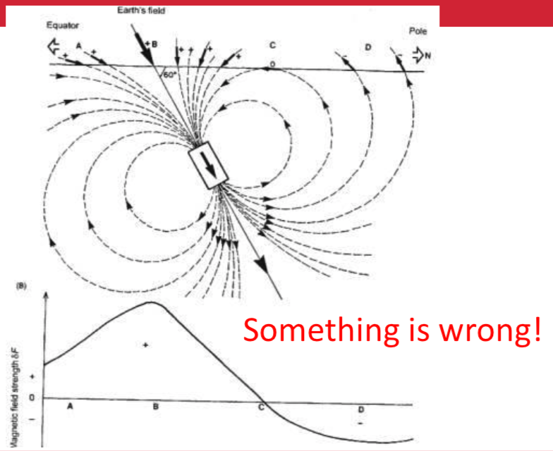
If Earth is a stationary non-rotating spherical body with uniform density distribution, the strength of gravitation acceleration would be constant over the surface. However, the Earth is rotating. The centrifugal force is created by the rotation of Earth and the gravitational force  is created from non-rotating Earth. Thus, the gravitational force and the centrifugal force combine to yield the observed gravitational force
  . Consequently, the Earth’s gravity field decreases from poles to equator.
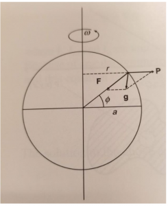 is centrifugal force. is gravitational force. is observed gravitational force.
2.4.4.2 Total gravity and theoretical gravity
The Earth’s gravity is due to both the mass of the Earth and the centrifugal force caused by Earth’s rotation, so the total potential is the sum of its self-gravitational potential  and its rotational potential
  . The equation of total gravity potential is below:
![\[U=U_g + U_r\]](https://uhlibraries.pressbooks.pub/app/uploads/quicklatex/quicklatex.com-9fd71ea5e037e632a148e6920c02fdbd_l3.png "Rendered by QuickLaTeX.com")
where,
![\[U_r=\frac12\omega^2r^2\cos^2\lambda\]](https://uhlibraries.pressbooks.pub/app/uploads/quicklatex/quicklatex.com-846cae16742b84ea4caaf14d637b23cb_l3.png "Rendered by QuickLaTeX.com")
 is angular velocity (
 ), is the axial radius and
  is latitude.
Theoretical gravity takes into account the effect of Earth’s spin on gravity. After gravity survey, the first thing we need to do is data processing. We need to remove the effects of general background (including the effect of Earth’s rotation) by subtracting theoretical gravity from measurements.
![\[g_0=g_e\left(1+\alpha\sin^2\lambda+\beta\sin^2\left(2\lambda\right)\right)\\\]](https://uhlibraries.pressbooks.pub/app/uploads/quicklatex/quicklatex.com-b98188c25ac60a201d99a921e2450a48_l3.png "Rendered by QuickLaTeX.com")
![\[g_0=g_e\left(\frac{1+k\sin^2\lambda}{\sqrt{1-e^2\sin^2\lambda}}\right)\\\]](https://uhlibraries.pressbooks.pub/app/uploads/quicklatex/quicklatex.com-b5676336f016ed8df4f20c0dd10bce00_l3.png "Rendered by QuickLaTeX.com")
where,  is gravitational attraction at equator.
Note that the theoretical gravity is the gravity due to a rotating and uniformly dense spheroid (i.e., an idealized and overly simplified Earth).
2.4.4.3 The shape of the Earth
As the Earth spins, the centrifugal force causes the Earth to bulge at the equator. So the Earth has a spheroidal shape. Spheroid is the surface obtained by rotating an ellipse about one of its principal axes. Spheroid is therefore an ellipsoid with two equal semi-axes. It has circular symmetry.
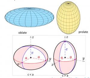
Therefore, the Earth is an oblate spheroid shape (seeing figure below) and the difference between the major axis and the minor axis around  km.
km.
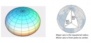
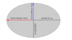
2.4.4.4 Reference ellipsoids and geodetic datums
Geodesists have adopted an ellipsoid model to determine latitude and longitude coordinates. There are a few such ellipsoid models, also called reference ellipsoids. Different ellipsoid models result in different geodetic datums.
A geodetic datum uniquely defines all locations on Earth with coordinates. Datums precisely specify each location on Earth’s surface in latitude and longitude. NAD27, NAD83, and WGS84 are geodetic systems. NAD27 uses the Clarke Ellipsoid of 1866. NAD83 is the most current datum being used in North America. It uses reference ellipsoid GRS80. It forms the basis of coordinates of all horizontal positions for Canada and the US. WGS84 is the reference coordinate system used by GPS. It uses the WGS84 ellipsoid.
Rotation plays a significant role in the Earth. Here, we briefly summarize the rotation:
(a) Rotation causes centrifugal forces, which causes gravity to decrease from poles to the equator.
(b) Rotation causes a difference between polar and equatorial radii, which yields a larger gravitational attraction at the poles compared with the equator (because of the smaller distance to the center).
(c) The combined centrifugal force and flattening effect results in a difference of approximately 5.3 mgal between gravity measurements at poles and equator.
2.4.5 Geoid
Before talking about geoid, let’s recall the relevant details about the equipotential surface.
An equipotential surface is a surface on which the potential remains constant. That is:
![\[\phi\left(x,y,z\right)=cons\tan t\\\]](https://uhlibraries.pressbooks.pub/app/uploads/quicklatex/quicklatex.com-10b31aa90524cc05514d77c52804d95f_l3.png "Rendered by QuickLaTeX.com")
Suppose  is a unit vector that is tangential to an equipotential surface of , then
![\[\mathbf{\widehat S}\cdot \mathbf{F}=\frac{\partial\phi}{\partial\mathbf{\widehat S}}=0\\\]](https://uhlibraries.pressbooks.pub/app/uploads/quicklatex/quicklatex.com-42de101399b4f7802179fdd4deb517e4_l3.png "Rendered by QuickLaTeX.com")
2.4.5.1 Basic concepts of geoid
(a) Geoid is an equipotential surface.
(b) The gravitational field is the norm to the geoid and defines the vertical direction at any location.
(c) Geoid is the equipotential surface that coincides with the mean ocean surface (or mean sea level) (assuming no tides, ocean currents, winds, etc.) and extends through the continents.
(d) The geoid at any point on land can be thought of as the level of water in an imaginary canal connected at each end with the ocean.
Here is a question. Why the mean ocean surface is an equipotential surface for the Earth’s gravitational field?
The figure above is the ocean. If the ocean is not an equipotential surface, there will be a horizontal component of the Earth’s gravitational field acting on the ocean water, which means gravity will move the ocean water. But in reality, ocean water is stationary (assuming no tides, winds). This phenomenon explains why the ocean is the equipotential surface.
Geoid is closely related to a spheroid. If the spheroid is rotating earth with uniform density, then the geoid and spheroid will coincide. However, we all know that the density within the Earth changes spatially. So, depending on the density distribution, the geoid will be higher or lower than the reference ellipsoid (shown in the figure below). In the figure below, we noticed that the ocean surface (number  ) is higher or lower than the reference ellipsoid (green dash line, the number
  ). For a local excess mass, geoid will be higher than the spheroid (i.e., warp outward) in order to keep the potential constant.
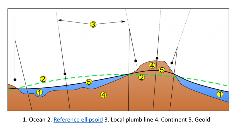 is the ocean surface. Number , green dash line, is the reference ellipsoid. Number
  is local plumb line. Number
  Continent, we can regard this as rock. Number
  is geoid.
2.4.5.2 Geoid undulations
Geoid undulations are the differences between geoid and ellipsoid. Seeing figure below:
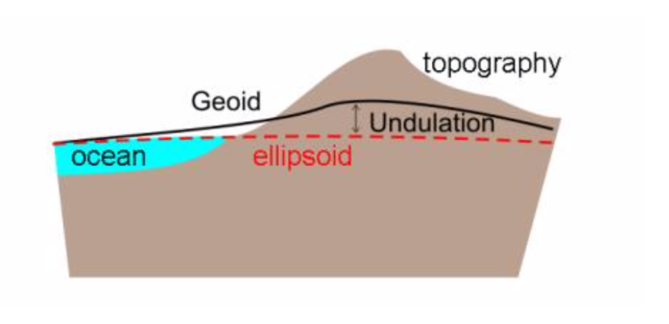
Here are some examples of geoid undulations. All of the figures have the same trend. The dark blue color is the area where geoid is lower than ellipsoid, which means something has a low density in this area. In comparison, red color is the area where geoid is higher than ellipsoid, which means the high density underneath this area.
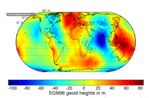
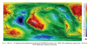
The heights obtained from GPS are typically ellipsoid height, which means the distance between point of interest and ellipsoid. The height displayed on most consumer handheld GPS receiver is, however, the orthometric height, height above mean sea level (LaFehr and Nabighian, 2012, P12s).
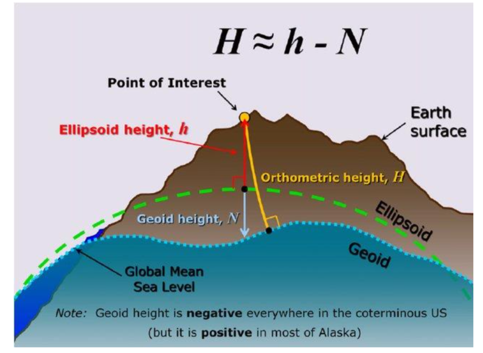
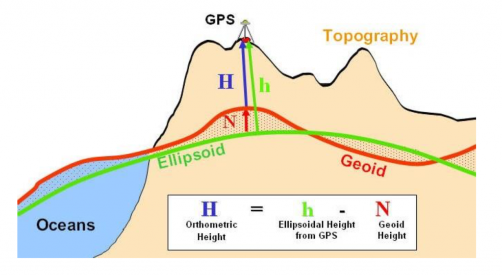
Here is an equation to compute orthometric height:
![\[H=h-N\]](https://uhlibraries.pressbooks.pub/app/uploads/quicklatex/quicklatex.com-21537612e43a06609f039d2bb585195f_l3.png "Rendered by QuickLaTeX.com")
 is orthometric height means the distance between the observation point to the geoid surface.
  is ellipsoidal height means the local plumb distance from the observation point to ellipsoid. The ellipsoidal height is currently obtained from a handheld GPS receiver.
  is the geoid height. The geoid height is negative when the geoid surface is lower than ellipsoid, and geoid height is positive when the geoid surface is higher than ellipsoid.
2.5 Gravitational Potential & Gravity Gradiometry
2.5.1 A few gravity examples
2.5.1.1 Unit of gravity attraction/acceleration
(a). In the International System ( ), mass has a unit of kilograms (
 ), distance is meters ().
(b). Gravitational acceleration  has a unit of
  . This is a very large unit to use. So, we use
  instead. The unit is also refereed to as
  (short for Galileo).
(c). Unit of gravitational constant is  .
.
Derivation
![\[\mathbf g(p)=-\gamma\frac m{r^2}\widehat{\mathbf {r}}\]](https://uhlibraries.pressbooks.pub/app/uploads/quicklatex/quicklatex.com-103784df1604a35c5b1ab8bdb1d2def9_l3.png "Rendered by QuickLaTeX.com")
If has a unit of , and has a unit of , and has a unit of . The unit of two sides is:
![\[\frac m{sec^2}=?\frac{kg}{m^2}\]](https://uhlibraries.pressbooks.pub/app/uploads/quicklatex/quicklatex.com-bb5ed78c0b81d73af66c593fca94e058_l3.png "Rendered by QuickLaTeX.com")
So, we obtain is  . The unit of is .
(d). is a more appropriate unit to use, but even is too large for geoscience applications, so we currently use  .
.
where,  .
.
(e). Sometimes, even is too large, in such cases, we use  .
.
where,  .
.
(g). Microgravity measures minute change in the earth’s gravitational filed, which can be used for time-lapse hydrogeophysical studies, aquifer recharge and depletion, fluid monitoring in a petroleum reservoir, fluid flow in geothermal reservoirs, underground cavities.
Microgravity
Not to be confused with microgravity experienced by astronauts in space, where microgravity is the condition in which people or objects appear to be weightless.
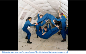
2.5.1.2 Examples
Example
is most common used unit in gravity measures. For global scale, the gravity anomalies is hundreds of . Seeing the figure below, the total range of color bar is  .
.
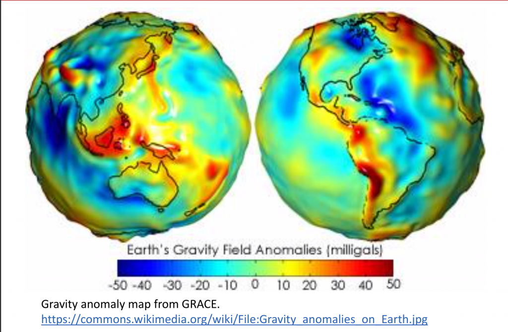
Example
The entire range of bouguer gravity anomalies is hundreds of , this range is widely used in geophysics, and we rarely use the . In gravity data processing, we firstly have to correct bouguer anomalies that will remove all effects of mountain and terrain. The warm color reflects high density, the cold color reflects low density. The  value here roughly corresponds to average density. In the New Jersey area, the highest feature is characterized as a Northeast to Southwest anomalies caused by basalt intrusion.
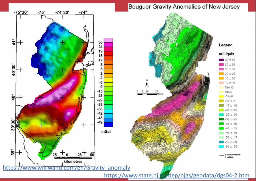
Example
The highest anomalies are closely related to mid continent rift, which means something subsurface has really high density.
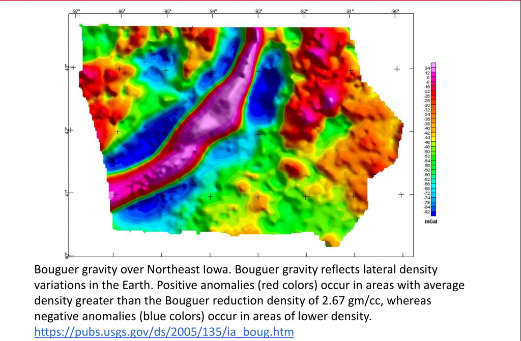
Example
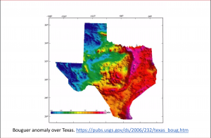
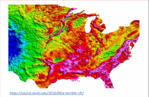
Bouguer anomaly over Texas (left) and bouguer anomaly over America.
Example
The figure below (left) is reduced-to-pole total field aeromagnetic anomalies. The figure below (right) is bouguer ground gravity data. The range of color bar for bouguer gravity is around , which is currently used in mineral exploration.
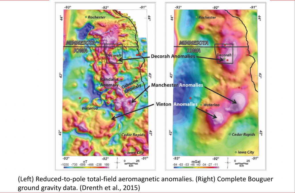
Example 
The figure below (left) is observed gravity data, the figure below (right) is geological model built based on drill hole data.
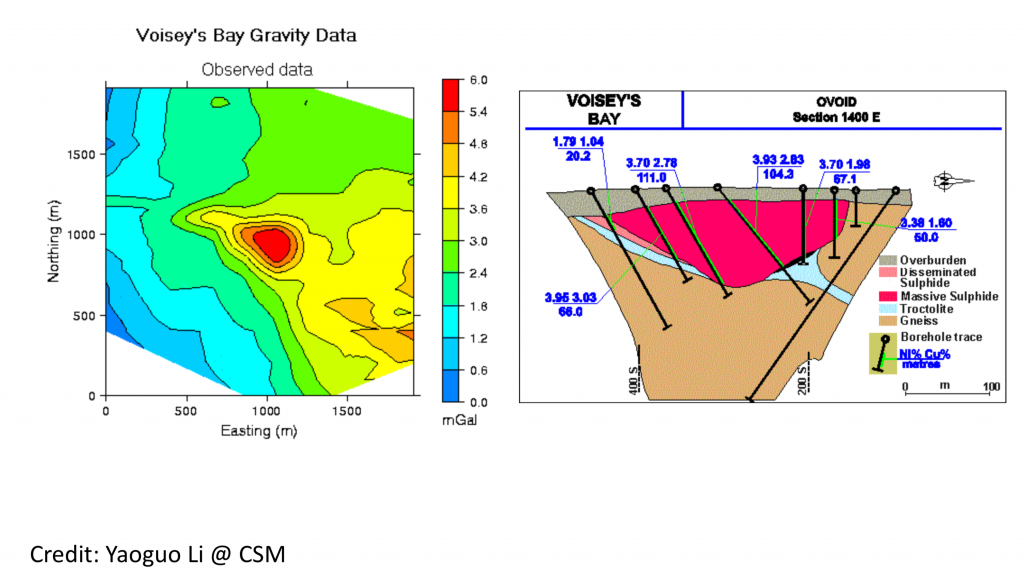
Example 
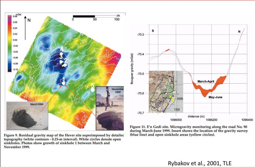
Example 
Time-lapsed gravity measure can be used to monitor fluid flow subsurface.
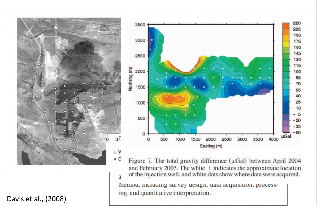
Example 
CG-5 is used to measure gravity anomaly in field camp.
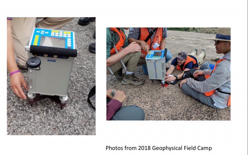
2.5.2 Gravity gradiometry
2.5.2.1 Basic Concepts of Gravity Gradiometry
Gravity gradiometry is defined as a measure of the spatial changes in gravitational acceleration g. In order to better understand gravity gradiometry, we must return to the concept of gravitational acceleration being a vector field. As a vector, g is composed of 3 components: gx, gy, and gz. Normally, the influence of the gx and gy components of gravity are minuscule and commonly disregarded in gravity surveys as most gravimeters measure gravity along the gz component. A spatial change of gz in the x-direction is defined as  which measures how fast gz changes in the x-direction. Similarly,
  and
and  describe the spatial change of gz in the y-direction and z-direction.
2.5.2.2 Gravity Gradiometry Tensor
The spatial change relationships listed above for gz also apply to gx and gy, resulting in 9 components that can be organized into the following tensor:
![\[T = \begin{Bmatrix} \frac{dg_x}{dx}\frac{dg_x}{dy}\frac{dg_x}{dz} \\ \frac{dg_y}{dx} \frac{dg_y}{dy} \frac{dg_y}{dz} \\ \frac{dg_z}{dx} \frac{dg_z}{dy} \frac{dg_z}{dz} \end{Bmatrix}\]](https://uhlibraries.pressbooks.pub/app/uploads/quicklatex/quicklatex.com-9eb0091cab47fda2ed233eca1df37969_l3.png "Rendered by QuickLaTeX.com")
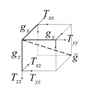
This can also be expressed in the simpler form of
![\[T = \nabla^Tg\]](https://uhlibraries.pressbooks.pub/app/uploads/quicklatex/quicklatex.com-f9bfedcba9ed4e031a07a27b74f86e0a_l3.png "Rendered by QuickLaTeX.com")
Recall that gravity is the gradient of gravitational potential:  . Therefore, the gravity gradient is the second order derivative of the gravitational potential and can be expressed as the following:
![\[T = \nabla \nabla^T \phi= \begin{Bmatrix} \frac{d^2 \phi}{dx^2}\frac{d^2 \phi}{dydx}\frac{d^2\phi}{dzdx} \\ \frac{d^2 \phi}{dxdy} \frac{d^2 \phi}{dy^2} \frac{d^2 \phi}{dzdy} \\ \frac{d^2 \phi}{dxdz} \frac{d^2 \phi}{dydz} \frac{d^2 \phi}{dz^2} \end{Bmatrix}\]](https://uhlibraries.pressbooks.pub/app/uploads/quicklatex/quicklatex.com-a21aace3a4d78edc8f716dac79145841_l3.png "Rendered by QuickLaTeX.com")
While the gravity gradient tensor may look complex with 9 components, there are a few important properties of gravitational potential that simplify the tensor down to only 5 independent components.
- Gravitational potential is well-behaved outside the source region and the tensor is therefore symmetric:
![\[\frac{d^2}{dxdy} = \frac{d^2}{dydx}, etc.\]](https://uhlibraries.pressbooks.pub/app/uploads/quicklatex/quicklatex.com-e4f3c2dca76984e094686e6df2d080bd_l3.png "Rendered by QuickLaTeX.com")
- The potential is harmonic outside the source region, meaning that the tensor has zero trace
 :
:
![\[\nabla^2\phi = 0\]](https://uhlibraries.pressbooks.pub/app/uploads/quicklatex/quicklatex.com-54459b9e239408e7d744b86f65ce9c93_l3.png "Rendered by QuickLaTeX.com")
As a reminder, the trace of a matrix is the sum of its elements along the main diagonal.
One example of the five independent components of the gravity gradient tensor is as follows:  and
and 
2.5.2.3 Units of Gravity Gradients
In order to find the units of gravity gradient measurements, we must first start with the units of gravity which is . The gravity gradient measures the spatial change in gravity over a short distance, meaning that it has a unit of  in SI units, or also
  and
and  . These units are normally too large to use, so units of Eotvos or Eö are used instead, with 1 eotvos =
  = 0.1 mGal/km = 0.1
  Gal/m. This is an extremely sensitive unit of measurement!
2.5.2.4 Calculating Gravity Gradient
In order to find the gravity gradient, we must first start with the equation of gravity due to a point source:
![\[g(P) = \gamma m \nabla \frac{1}{r}\]](https://uhlibraries.pressbooks.pub/app/uploads/quicklatex/quicklatex.com-2613fb045c7a0ad9f107c2019461f295_l3.png "Rendered by QuickLaTeX.com")
Recall that 
The gravity gradient of a point source can therefore be represented as:
![\[T = \gamma m \nabla \nabla ^T \frac{1}{r}\]](https://uhlibraries.pressbooks.pub/app/uploads/quicklatex/quicklatex.com-d5dfe2892cd27541de5df46cfc09c55f_l3.png "Rendered by QuickLaTeX.com")
In the general case, gravity gradient can be expressed as:
![\[T = \gamma m \nabla \nabla ^T \frac{\vec{1}}{|\vec{r} - \vec{r'}|}\]](https://uhlibraries.pressbooks.pub/app/uploads/quicklatex/quicklatex.com-f8c3b96a11058a18be44ad0d14e5e4d8_l3.png "Rendered by QuickLaTeX.com")
As an example, we will now take a look at the equation for gravity gradient at  :
:
![\[T_{xx} = \gamma m \frac{2(x-x')^2-(y-y')^2 - (z-z')^2}{[(x-x')^2+(y-y')^2 + (z-z')^2]^{5/2}}\]](https://uhlibraries.pressbooks.pub/app/uploads/quicklatex/quicklatex.com-aaeeee175bb616b1b3a9433f897e1c13_l3.png "Rendered by QuickLaTeX.com")
Additionally,  is represented below:
![\[T_{xz} = \gamma m \frac{3(x-x')(z-z')}{[(x-x')^2+(y-y')^2 + (z-z')^2]^{5/2}}\]](https://uhlibraries.pressbooks.pub/app/uploads/quicklatex/quicklatex.com-6d2ffef07e8dcc61a96452eb4766dded_l3.png "Rendered by QuickLaTeX.com")
Notes:
We will see  again later in regards to the magnetic field due to a small current loop!
Additionally, T and G are interchangeable representations of gravity gradient.
2.5.2.4 Examples
Example
The image below is of the gravity and gravity gradient responses to an anomaly in the subsurface.  is the gravity response of the body, while all components of
  represent the gravity gradient response. Notice that
  is easier to interpret compared to the other components of the gravity gradient.
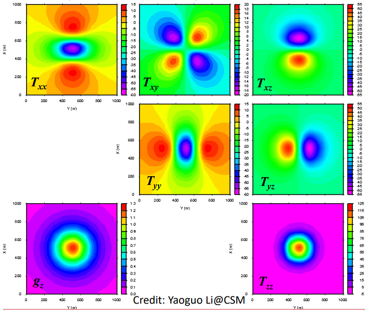
Synthetic Gravity Gradient Data. The gravity gradient data is in units of Eotvos and the gravity data is in units of
Example
Vertical gravity and gravity gradient signals from a point source buried at 1km depth. While the two signals do not share the same units, notice that the responses of and  are fairly similar, although the signal of is narrower and better constrained over the anomaly.
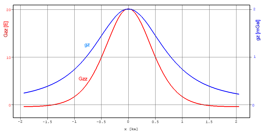
Example
Notice the difference between the collected Bouguer gravity and component gravity gradient data collected over the same region. The boundaries of different anomalies in are better defined than in the Bouguer gravity data. AGG stands for Airborne Gravity Gradiometry.
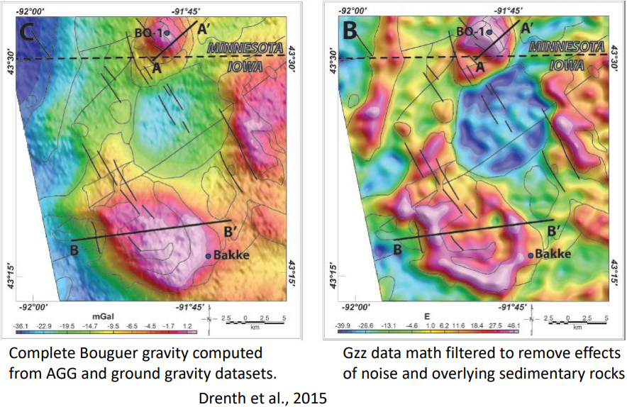
Example
Falcon gravity gradient map ( ) of the western Eyasi rift basin. A 3D model of the area was produced by combining the responses from the Falcon AGG and airborne magnetic data. Basement structural features and sediment depo-centers are easily identified in the model.
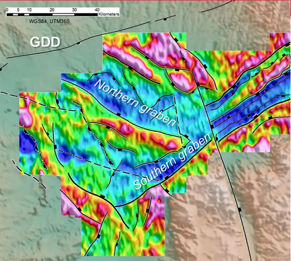
Example
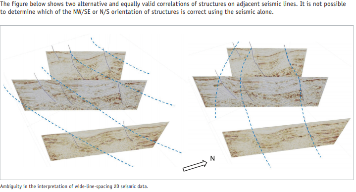
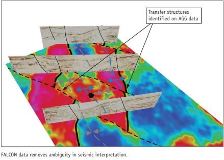
Example
Both figures below are gravity gradiometry surveys conducted over the Vinton Salt dome.
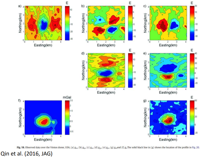
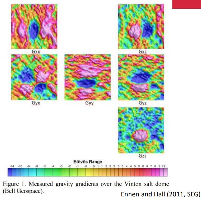
Example
Another gravity gradiometry figure of the Vinton salt dome, but note the error made with the units.
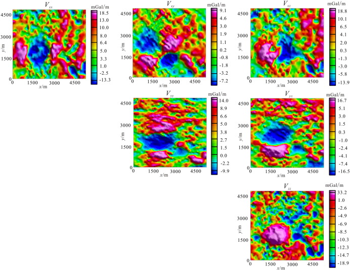
2.6. MAGNETIC POTENTIAL
2.6.1. BIOT-SAVART LAW
From classical electromagnetism, we know that electricity and magnetism are inter-related. For example, if we have a wire of current, it will generate a magnetic field, as illustrated in the figure below.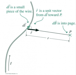
In order to calculate the current in the wire which induced the magnetism, we can use Biot-Savart law, which is mathematically written as follows:
![\[d\Beta =\frac{{{\mu }_{0}}}{4\pi }\frac{Idl\times \mathbf{\hat{r}}}{{{r}^{2}}}\]](https://uhlibraries.pressbooks.pub/app/uploads/quicklatex/quicklatex.com-be6e6e0e83e7c3d5565f6116b2787302_l3.png "Rendered by QuickLaTeX.com")
Integrating around a loop  yields the following expression:
![\[\mathbf{B}=\frac{{{\mu }_{0}}}{4\pi }{{I}_{b}}\oint{\frac{d{{l}_{b}}\times\mathbf{\hat{r}}}{{{r}^{2}}}}\]](https://uhlibraries.pressbooks.pub/app/uploads/quicklatex/quicklatex.com-edeb790a0bc25bb2298d31f77e844008_l3.png "Rendered by QuickLaTeX.com")
Where  is the magnetic constant permeability of the vacuum (free space),
  is the “current element” directed along the current in the wire, the unit vector
  is pointing from the current element towards the observation point where the magnetic field
  is to be calculated. Magnetic field vector induced at observation location P due to the steady current in the wire is at right angles to both and , and its direction can be determined through the Right-Hand Rule.
The magnetic field of a loop of current can be called as
- Magnetic induction
- Magnetic flux density
- Magnetic field
2.6.1.1.1 Right-hand rule
The directions of the current and magnetism can be represented by our right hand. As shown in the figure, we can point the right thumb in the direction of the current, then curl your figures to get the magnetic field directions.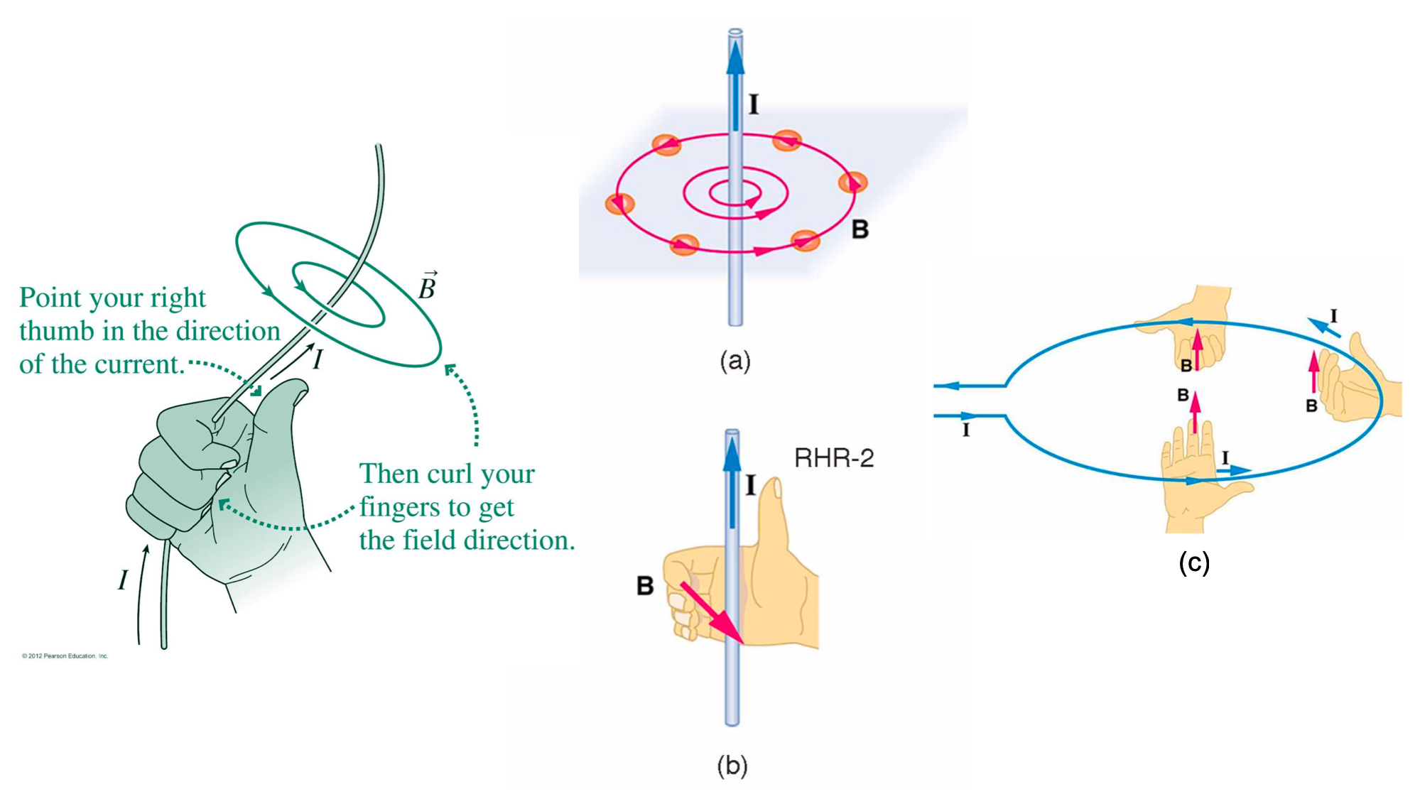
2.6.1.1.2 Magnetic field unit
The SI unit for the magnetic field is Tesla denoted as . However, this unit is too large to represent the actual field measurements. Therefore, we often use nanotesla ( ) instead, where
![\[1nT={{10}^{-9}}T\\]](https://uhlibraries.pressbooks.pub/app/uploads/quicklatex/quicklatex.com-d595d393c3accbe98eecb6ca0ef701ef_l3.png "Rendered by QuickLaTeX.com")
The Iowa magnetic anomaly map is shown here to demonstrate the value range of the measured magnetic field data, which is about 1300 nT for a regional-scale study area. If in the explorational scale, the range value would be even smaller.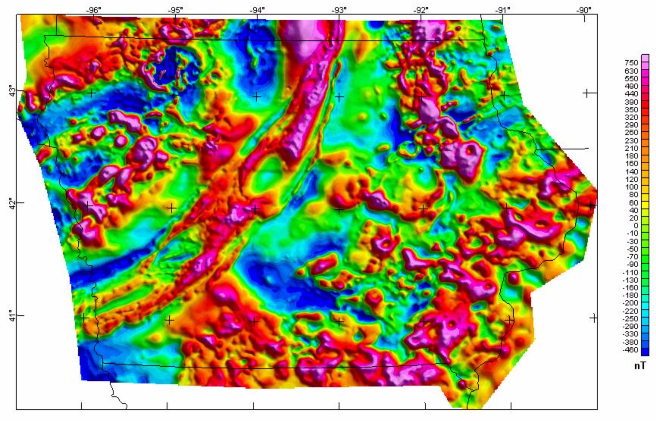
2.6.1.1.3 Implications from Helmholtz Theorem
Before we move on to the magnetic potentials, let us be reminded about the consequences of the Helmholtz theorem. We have learned that a vector field is a solenoidal field in a region if its divergence vanishes everywhere, i.e.,
![\[\nabla \cdot \mathbf{F}=0\]](https://uhlibraries.pressbooks.pub/app/uploads/quicklatex/quicklatex.com-a8701149603e81fd237bc96a79d28498_l3.png "Rendered by QuickLaTeX.com")
According to the Helmholtz theorem, the scalar potential becomes zero. Therefore,
![\[\mathbf{F}=\nabla \times \mathbf{A}\]](https://uhlibraries.pressbooks.pub/app/uploads/quicklatex/quicklatex.com-92f07fa3e0b85baab3fb72d9c22656b6_l3.png "Rendered by QuickLaTeX.com")
An example of the solenoidal field is the static magnetic field, i.e., a magnetic field that does not change with time. As illustrated in the (figure), magnetic field lines do not emanate from or converge to any point, and since there is no source, these field lines are closed loops. Therefore, its divergence is zero, and magnetic field is solenoidal
![\[\nabla \cdot \mathbf{B}=0\]](https://uhlibraries.pressbooks.pub/app/uploads/quicklatex/quicklatex.com-a006feeaf7dbebb3bbd4228db46e2ef5_l3.png "Rendered by QuickLaTeX.com")
This statement is true everywhere, even within magnetic media.
If applying divergence theorem, we will have an equation as follows:
![\[\oint{\nabla \cdot \mathbf{B}}dv=\oint\limits_{S}{\mathbf{B}}\cdot \mathbf{\hat{n}}ds=0\]](https://uhlibraries.pressbooks.pub/app/uploads/quicklatex/quicklatex.com-57c5cb40cfba9f291429b7365da1f1a4_l3.png "Rendered by QuickLaTeX.com")
It implies that the net magnetic flux over any closed surface is always zero. And there are no net sources (or sinks) anywhere in the space. Therefore, magnetic monopole does not exist. These implications are demonstrated in the figure below, where all magnetic field lines entering and exiting the shaded area no matter how many field lines there are. Thus, there is no magnetic volume.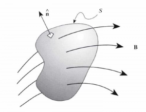
Furthermore, according to Helmholtz theorem, we will then have
![\[\mathbf{B}=\nabla \times \mathbf{A}\]](https://uhlibraries.pressbooks.pub/app/uploads/quicklatex/quicklatex.com-d9359d78d3d5042c053b8ea5a467959d_l3.png "Rendered by QuickLaTeX.com")
Where  is a vector potential and always exists.
However, under certain circumstances, the scalar potential for the magnetic field also exists at the same time (note that vector potential still always exists). In order to explain this phenomenon, we need to review the Ampere’s Law.
2.6.1.2. Ampere’s Law
In the previous section, you see Biot-Savart law that gives you the equation of the magnetic field (B), which is the following:
![\[\mathbf{B}=\int{\frac{{{\mu }_{0}}}{4\pi }}\frac{dl\times \mathbf{\hat{r}}}{{{r}^{2}}}\]](https://uhlibraries.pressbooks.pub/app/uploads/quicklatex/quicklatex.com-4be5795eccb25eb6db4abb8003fb3f87_l3.png "Rendered by QuickLaTeX.com")
Ampere’s law gives the following relation between magnetic field B and current density j:
![\[\nabla \times B = \mu_0 j\]](https://uhlibraries.pressbooks.pub/app/uploads/quicklatex/quicklatex.com-615a1c3a391650fa648435bdafb7c63f_l3.png "Rendered by QuickLaTeX.com")
Both the Biot-Savart and Ampere’s law essentially expresses the same concept but in different forms. Both equations tell us that if you have current, then you will have a magnetic field (and vice versa).
To learn more about how to derive Ampere’s law from Biot-Savart law, please refer to Page 229-233 in David J. Griffith’s book (Introduction to Electrodynamics, Fourth Edition).
Note that j in Ampere’s law refers to the total current density, which consists of three parts: free current( ), bound current (
 ), and magnetization current (
 ). The division between the current densities are not so relevant for this chapter, but if you wish to learn more about this topic, you can do so through this link.
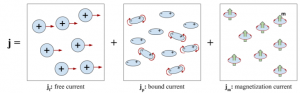
However, a question arises from Ampere’s law, what if there is no current? Putting it on the perspective of Ampere’s law, if there is no current in the region of investigation, then this holds true:
![\[\nabla \times B = 0\]](https://uhlibraries.pressbooks.pub/app/uploads/quicklatex/quicklatex.com-d2c018ff31ab11ee2b7161a354c32f00_l3.png "Rendered by QuickLaTeX.com")
This implies that the divergence of the magnetic field, and thus B is irrotational. Recall Helmholtz theorem. If B is irrotational, then that means there exists a scalar potential V that satisfies  .
.
The above equation is only true if the region of study does not have currents. In many geophysical situations, electrical currents are negligible in regions where the magnetic field is measured. Therefore, in general, the scalar potential exists outside of magnetic materials. This is good news for geophysics applications because we do not have to worry about dealing with vector potentials (which is more complicated). We just need to derive the scalar potential to get B! This can be done by deriving the scalar potential V and then taking the negative gradient ().
2.6.2. magnetic field due to the magnetic dipole
In this section, we will talk more about magnetic dipoles and how it can help us find the scalar potential of the magnetic field.
2.6.2.1 Magnetic Field due to a Small Loop
When we talk about the magnetic field due to a small loop, we are talking about the magnetic field outside of the loop, and therefore the scalar potential exists. The basic strategy, in this case, is to derive the scalar potential first. 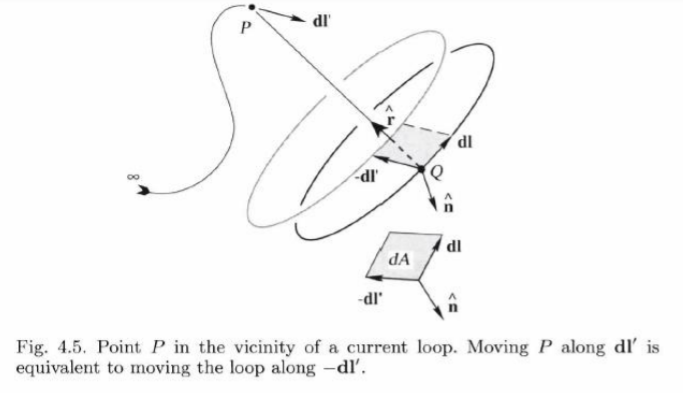
The potential change caused by moving the test particle Q along with the line segment dl’ is:
![\[dV(P) = -B . dl'\]](https://uhlibraries.pressbooks.pub/app/uploads/quicklatex/quicklatex.com-9212af4146a6abd9fa2394c75a2a4415_l3.png "Rendered by QuickLaTeX.com")
where B is the magnetic field due to the loop. Recall Biot-Savart law:
![\[B = \frac{\mu_0}{4\pi} I \oint \frac{dl \times \hat{r}}{r^2}\]](https://uhlibraries.pressbooks.pub/app/uploads/quicklatex/quicklatex.com-d95b7c159e9c9e6e0bcf4f0d773bd81a_l3.png "Rendered by QuickLaTeX.com")
Substituting B from Biot-Savart can give us:
![\[dV(P) = -\frac{\mu_0}{4\pi} I \oint \frac{dl \times \hat{r}}{r^2} . dl'\]](https://uhlibraries.pressbooks.pub/app/uploads/quicklatex/quicklatex.com-6685104bbd6f383b300c5a3ae166900d_l3.png "Rendered by QuickLaTeX.com")
Where  is a constant and can be moved inside the integral. Also, use the vector identity
  . Thus, the equation becomes:
![\[dV(P) = -\frac{\mu_0}{4\pi} I \oint \frac{dl \times (-dl') . \hat{r}}{r^2}\]](https://uhlibraries.pressbooks.pub/app/uploads/quicklatex/quicklatex.com-8ae0d7f4d68bb3ff70709f41c5f5e073_l3.png "Rendered by QuickLaTeX.com")
We introduce the concept of solid angle( ), which is the solid angle subtended at P by the entire ribbon of wire. In geometry, a solid angle is a measure of the amount of the field of view from some particular point that a given object covers. That is, it is a measure of how large the object appears to an observer looking from that point. The point from which the object is viewed is called the apex of the solid angle, and the object is said to subtend its solid angle from that point.
Thus, the equation can then be rewritten into:
![\[dV(P) = \frac{\mu_0}{4\pi} I d\Omega\]](https://uhlibraries.pressbooks.pub/app/uploads/quicklatex/quicklatex.com-a0043515b537da202d0ebc13fe4ffec6_l3.png "Rendered by QuickLaTeX.com")
If we assume that the loop is very small in diameter compared to r, we do not need to use the integral. Otherwise, we would need to use the integrals for the solid angle. Thus, with this assumption, the following equation for the magnetic scalar potential due to a small loop can be rewritten as:
![\[V(P) = \frac{\mu_0}{4\pi} I \frac{\hat{n} . \hat{r}}{r^2} \Delta S\]](https://uhlibraries.pressbooks.pub/app/uploads/quicklatex/quicklatex.com-9ad78216823fc7feff7c053228276385_l3.png "Rendered by QuickLaTeX.com")
Where  is the area of the loop, and
  is the normal vector of that area.
Now, let us define the dipole moment (a vector),mathematically expressed as such:
![\[m = I \Delta s \hat{n}\]](https://uhlibraries.pressbooks.pub/app/uploads/quicklatex/quicklatex.com-e885de779f7dd3b82cd5a627fd4dded8_l3.png "Rendered by QuickLaTeX.com")
The equation for the scalar potential in terms of dipole moment (m) is then:
![\[V(P) = \frac{\mu_0}{4\pi} \frac{m . \hat{r}}{r^2} = -\frac{\mu_0}{4\pi} m . \nabla_p \frac{1}{r}\]](https://uhlibraries.pressbooks.pub/app/uploads/quicklatex/quicklatex.com-388b96590ff12ed3d2f09cf8f3ae7027_l3.png "Rendered by QuickLaTeX.com")
![\[V(P) = \frac{\mu_0}{4\pi} \frac{m . \hat{r}}{ r^2}\]](https://uhlibraries.pressbooks.pub/app/uploads/quicklatex/quicklatex.com-7e1ce3c74c5c6c7733ddffb90f980574_l3.png "Rendered by QuickLaTeX.com")
The above equation implies that the function decays as the square of distance. Recall that gravity field also decays as the function of square of distance (1/ ), while the gravitational potential decays as a function of distance (1/). This means, given a fixed dipole moment, the potential value depends on the distance and . The potential is positive when the angle between m and is smaller than
  , and negative when the angle is larger than .
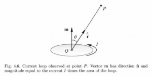
The following pictures will help you understand the signs of the potential field value better. Suppose the current loop is placed in the middle (origin) of the following picture and the dipole moment is pointing to the North. Then if you place your point P in any of the regions, the color of the region in the picture below tells you the sign of potential due to the magnetic dipole in point P. In the picture, red indicates more positive values and blue indicates more negative values.
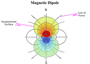
From the above picture, we can see that:
- V(P) is positive(+) if the angle between m and is <90 degrees.
- V(P) is negative(-) if the angle between m and is >90 degrees.
- V(P) is zero(0) if the angle between m and is 90 degrees.
For example, we can see that the smallest potential value is achieved when the angle is between m and is  (the most negative you can get).
Test your understanding
From the picture below, where the color bar represents potential, can you tell where the direction of the dipole moment (m) is?
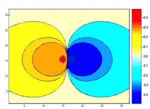
2.6.2.1 Depth Estimation with Magnetic Dipoles
Suppose a magnetic dipole is buried underground, and you are tasked to figure out the depth of it. We can do so by measuring the field response.
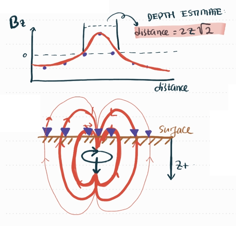
For example, in the above figure, we have a magnetic dipole buried underground and oriented downwards such that the magnetic field lines are oriented vertically. Suppose the blue triangles represent the observation location, which measurements are recorded in the Bz graph above it. The interaction between the field lines that hits the observation location (blue triangle) with the direction of the positive Z axis (pointing downwards) is what is recorded in the Bz graph. For example, the observation station on the left-most side has the field line pointing approximately upwards, and the positive Z axis is pointing downwards. Adding the two directions will lead to having a negative reading in Bz. There are two points in the above figure where the field lines are perfectly orthogonal (the two blue triangles next to the middle triangle) with the positive Z-axis, and thus the measurement of Bz is 0. Lastly, the observation right in the middle of the dipole experiences the most positive Bz because the field lines are in the same direction as the positive Z-axis. This leads to the profile we see in the graph.
It turns out the distance between the zero-crossing in the Bz graph is proportional to the depth of the dipole, specifically, the distance between the two zero-crossing is proportional to  where is the depth of the dipole.
Similarly, if we have a dipole oriented in the horizontal direction (so the field lines are mostly pointing horizontally), we can find the same response between the positive x axis with the field lines to create the graph for Bx. In this case, the distance between the zero-crossings are exactly the same as  , where z is the depth of the horizontally-oriented dipole.
Below are other orientation of the dipoles and the relation between the zero-crossing in the graph with the depth (z) of the magnetic dipole.
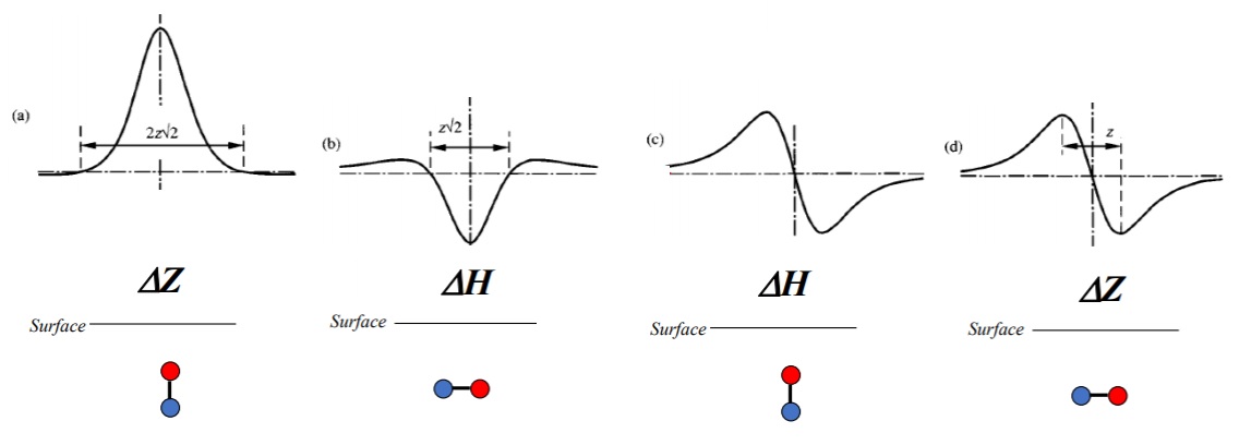
 ) and Bz (
 ) from different orientation of the magnetic dipole (two connected circles below the surface)
The above figure tells us that the broadness of the contours and profiles depends on the depth of the dipole ad provides a way of estimating the depth to the source. Please note that the above approximation is only true when we have a single magnetic dipole underground. There will be more complicated calculations involved for more complex cases. However, this approximation is still useful in certain cases. For example, even today we approximate the magnetic response from a seamount is approximately that of a single dipole moment. The shape of the anomaly depends on the shape of the seamount and the direction of the mean magnetization vector.
2.7. MAGNETIZATION
We have learned and derived the magnetic field due to a magnetic dipole (i.e., a vanishingly small loop of electrical current). However, this is not very realistic compared to real-life problems. Thus the question is asked: How about the magnetic field due to a volume of magnetic materials? You might have guessed it already, but the field due to a volume of magnetic material is the sum of the magnetic effects of all dipoles within that volume.
We define magnetization as the amount of dipoles within a certain volume. Mathematically expressed as:
![\[M = \frac{1}{V} \sum_i m_i\]](https://uhlibraries.pressbooks.pub/app/uploads/quicklatex/quicklatex.com-e91e8417c8a59f78916fb5c560ae90b6_l3.png "Rendered by QuickLaTeX.com")
Thus, magnetization is the vector sum of all individual dipole moments ( ) divided by the volume (V).
From the above equation, we can tell that the unit of magnetization is Ampere per meters (A/m).
2.7.1 MAGNETIC FIELD DUE TO A VOLUME
Before we sum the magnetic effects of all dipoles, we need to figure out the magnetic effects of only a tiny portion of the volume. So the question is: what is the magnetic field due to a small volume (dv)?
First, recall that the magnetic potential due to small dipole at a certain point (P) is the following:
![\[V(P) = -\frac{\mu_0}{4\pi} m . \nabla_p \frac{1}{r}\]](https://uhlibraries.pressbooks.pub/app/uploads/quicklatex/quicklatex.com-11d1f50caee3ef73f6d423df9f2789c2_l3.png "Rendered by QuickLaTeX.com")
Recall also that the equation for magnetization is:
Thus, rearranging the equation, we can see that the amount of dipoles(m) within a certain small volume (dV), is equivalent to M.dV.
![\[m = M dv\]](https://uhlibraries.pressbooks.pub/app/uploads/quicklatex/quicklatex.com-e2aaedf1c0b72890be8781f786c2fef9_l3.png "Rendered by QuickLaTeX.com")
That means, the magnetic potential due to a tiny volume is:
![\[dV(P) = -\frac{\mu_0}{4\pi} M . \nabla_p \frac{1}{r} dv\]](https://uhlibraries.pressbooks.pub/app/uploads/quicklatex/quicklatex.com-f40e706508e35cf85e1d3bbb89362958_l3.png "Rendered by QuickLaTeX.com")
Note the difference between dV and dv! Remember that dV is the magnetic potential due to a tiny volume and dv is the tiny volume of magnetic material.
What about magnetic potential due to big volume? Since a big volume consists of many tiny volumes, then we can sum/integrate them to obtain:
![\[V(P) = -\frac{\mu_0}{4\pi} \int_{vol} M(Q). \nabla_p \frac{1}{r} dv\]](https://uhlibraries.pressbooks.pub/app/uploads/quicklatex/quicklatex.com-d8fe65d47ba82be377a5a0d549e0c0dc_l3.png "Rendered by QuickLaTeX.com")
Where Q is the position of dv, and P is the position of observation.
![\[\nabla_p \frac{1}{r} = -\nabla_Q \frac{1}{r}\]](https://uhlibraries.pressbooks.pub/app/uploads/quicklatex/quicklatex.com-bd15f94f6a844b309acd8a7953b24c6a_l3.png "Rendered by QuickLaTeX.com")
where:
![\[r = \sqrt{(x_p-x_q)^2 + (y_p-y_q)^2 + (z_p-z_q)^2}\]](https://uhlibraries.pressbooks.pub/app/uploads/quicklatex/quicklatex.com-87039d6d0679d9af4e7511ead3380df6_l3.png "Rendered by QuickLaTeX.com")
With the above identity, we can then rearrange the equation as:
![\[V(P) = \frac{\mu_0}{4\pi} \int_{vol} M(Q). \nabla_Q \frac{1}{r} dv\]](https://uhlibraries.pressbooks.pub/app/uploads/quicklatex/quicklatex.com-9f26736749793d6e00bb52949814d132_l3.png "Rendered by QuickLaTeX.com")
Thus, the magnetic field due to a big volume would be:
![\[B(P) = -\nabla_P V(P) = -\frac{\mu_0}{4\pi} \nabla_P \int_{vol} M(Q). \nabla_Q \frac{1}{r} dv\]](https://uhlibraries.pressbooks.pub/app/uploads/quicklatex/quicklatex.com-a7926fe761aea8f03f95d4b4f7a0bf2c_l3.png "Rendered by QuickLaTeX.com")
2.7.2 MAGNETIC FIELD INTENSITY
2.7.2.1 Total Current Density
Recall Ampere’s law which is:
where j is the total current density consisting of free current (), bound current (), and magnetization current (). Thus, with the different parts of total current density, Ampere’s Law can also be expressed as:
![\[\nabla \times B = \mu_0 (j_m + \nabla \times M + \frac{\partial D}{\partial t})\]](https://uhlibraries.pressbooks.pub/app/uploads/quicklatex/quicklatex.com-aceec68eb0c0a72ceb774e43372bc0c4_l3.png "Rendered by QuickLaTeX.com")
Each part has the following meaning:
- : macroscopic currents (e.g., free current caused by moving charges)
 : magnetization currents due to the motion of electrons in atoms
 : displacement currents (can be ignored for most geophysical applications)
Knowing so, we can also write Ampere’s law as:
![\[\nabla \times B = \mu_0 (j_m + \nabla \times M)\]](https://uhlibraries.pressbooks.pub/app/uploads/quicklatex/quicklatex.com-6606e2bd605fae89c750fd4c730408c1_l3.png "Rendered by QuickLaTeX.com")
2.7.2.2 Magnetization Current
When exposed to an external magnetic field, the dipoles will align themselves accordingly. If the dipoles are all parallel to each other and have identical magnitude, circulating current of one dipole will cancel the current of its neighboring dipoles, resulting in a net surface current. If the magnetization is not uniform, a volume current will exist where circulating elemental currents fail to cancel.
To understand this concept, take a look at the Figure below. The dipoles are all oriented in the same direction and are uniform throughout the volume. The current inside the volume will cancel each other out, and thus leaving the outside volume to have a surface current (pictured ont he right), which in this case is counter-clockwise.
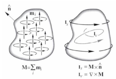
With simple mathematical arrangements:
![\[\nabla \times B = \mu_0 (j_m + \nabla \times M)\]](https://uhlibraries.pressbooks.pub/app/uploads/quicklatex/quicklatex.com-c7bb776913a9a5e4c8671ccf777923a2_l3.png "Rendered by QuickLaTeX.com")
We move  to the left hand side:
![\[\nabla \times \frac{B}{\mu_0} = j_m + \nabla \times M\]](https://uhlibraries.pressbooks.pub/app/uploads/quicklatex/quicklatex.com-f7c5baa86d44d3809bb847605c279740_l3.png "Rendered by QuickLaTeX.com")
Then, we move M to the left hand side:
![\[\nabla \times (\frac{B}{\mu_0} - M)= j_m\]](https://uhlibraries.pressbooks.pub/app/uploads/quicklatex/quicklatex.com-5752e69dc27f859dc7520bd7d4d5b03a_l3.png "Rendered by QuickLaTeX.com")
We can then define the following:
![\[H = \frac{B}{\mu_0} - M\]](https://uhlibraries.pressbooks.pub/app/uploads/quicklatex/quicklatex.com-00dcd587623b96423df438b4e1b445a7_l3.png "Rendered by QuickLaTeX.com")
To form the following:
![\[\nabla \times H = j_m\]](https://uhlibraries.pressbooks.pub/app/uploads/quicklatex/quicklatex.com-38e8605c3aa2a19ffe3e354ea0a12904_l3.png "Rendered by QuickLaTeX.com")
2.7.2.3 Magnetization Field Intensity
As previously stated, the magnetic field intensity (H) is mathematically defined as:
Magnetic field intensity is a hybrid vector with two components with quite different physical meanings.
The major difference between B (magnetic induction) and H (magnetic field intensity) is that the former originates from both free currents (macroscopic) and magnetization currents (atomic), as summarized by the following equation
whereas the latter arises only from true currents, as shown by the following equation.
![\[\nabla\times\matbhf{H} = \mathbf{j}_m\]](https://uhlibraries.pressbooks.pub/app/uploads/quicklatex/quicklatex.com-94014534dc0897c512950c224c446106_l3.png "Rendered by QuickLaTeX.com")
Also, be noted that magnetization M is subtracted from the definition of H. In other words, magnetization currents are excluded from the definition of magnetic field intensity, leaving behind only macroscopic currents.
Therefore, we can understand H as magnetic induction (except for a factor ) minus the effects of magnetization (M).
Outside of the magnetic materials, It holds true that  .
.
2.7.2.4 Magnetic scalar potential
According to Amphere’s law,
In the absence of such currents, we have:
![\[\nabla \times H = 0\]](https://uhlibraries.pressbooks.pub/app/uploads/quicklatex/quicklatex.com-fc3bfde3bd7e678299d1071c3b385f8a_l3.png "Rendered by QuickLaTeX.com")
Thus a scalar potential exists such that:
![\[H = -\nabla V'\]](https://uhlibraries.pressbooks.pub/app/uploads/quicklatex/quicklatex.com-7d5a99bfa035ac802a4f1729b7b88501_l3.png "Rendered by QuickLaTeX.com")
2.7.2.5 Magnetized Materials
Magnetic materials can be magnetized in the presence of an external magnetic field. What we mean by magnetized is that the dipole moments are aligned instead of randomly distributed. Mathematically this means:
![\[M = \frac{1}{V} \sum_i m_i \neq 0\]](https://uhlibraries.pressbooks.pub/app/uploads/quicklatex/quicklatex.com-46eb7a8a058c66896b6142a210390940_l3.png "Rendered by QuickLaTeX.com")
In the following picture, we see the difference between a non-magnetized (a) and magnetized (b) material. In the non-magnetized material, the arrows representing the dipoles are randomly oriented, and both H and M are zero. On the other hand, magnetized materials have the dipoles generally pointing on the same direction. In this case, the material is magnetized by an external field H pointing to the right, and M (which is a product of a material constant  and H) is also pointing to the right. This leads to the magnetic dipoles () pointing generally also to the right.
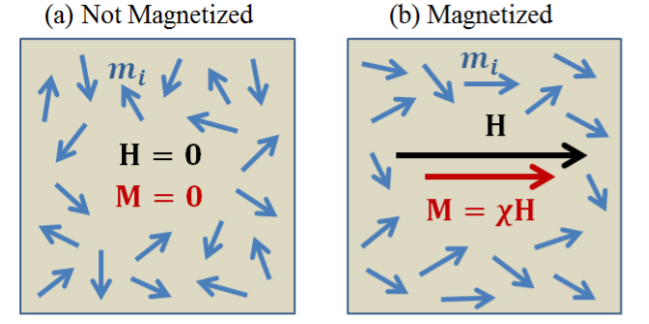
2.7.3 Induced magnetization
In the section below, we will cover induced magnetization and a couple of the properties associated with it. A couple key concepts that must be understood first include when a volume of magnetic materials acquires a non-zero net magnetization due to an external field, this is called induced magnetization. The external magnetic field applying the magnetization is called the inducing field.
2.7.3.1 Magnetic Susceptibility
When an inducing magnetic field (H) is applied to a material, the resulting induced magnetization (M) an be determined based the material’s magnetic susceptibility ( or
or  ). Magnetic susceptibility defines how easily a material (e.g., a rock) becomes magnetized under an inducing field and is unitless. The following equation describes this relationship:
![\[M = \kappa H\]](https://uhlibraries.pressbooks.pub/app/uploads/quicklatex/quicklatex.com-57f7450dfd54344c7f88a58c7d3ff0b3_l3.png "Rendered by QuickLaTeX.com")
.
However, this relationship is only true for low-amplitude inducing fields such as the Earth’s magnetic field.
From the relationship above, it’s clear that materials with high magnetic susceptibilities will also generate strong magnetic signals. In a geological context, magnetite-rich rocks are usually the main source of magnetic signals. However, in engineering buried metal objects such as water pipes are usually the sources for magnetic signatures. It is important to note that magnetic susceptibility can be positive or negative, and this will be covered in a following section on the types of magnetization.
Earth’s Magnetic Field
https://gpg.geosci.xyz/content/magnetics/magnetics_physical_property.html
- The Earth’s magnetic field is an inducing field
- Earth’s magnetic field is not uniform and will vary depending on location
- Objects will get magnetized differently depending upon where it is situated
- For example, the magnetic signals generated by a steel drum buried at the North pole will be very different compared to an equivalent drum buried at the equator.
Geologic Relationships of Magnetic Susceptibility
Blakely, 1996, p90
- In general, mafic rocks are more magnetic than silicic rocks
- Basalts are usually more magnetic than rhyolites
- Gabbros are usually more magnetic than granites
- Extrusive rocks generally have higher remanent magnetization and lower magnetic susceptibility than an intrusive rock of the same composition
- Sedimentary and metamorphic rocks often have low remanent magnetizations and magnetic susceptibilities
2.7.3.2 Magnetic Permeability
Magnetic permeability describes the ease at which magnetic flux can pass through a material, similar to how electric conductivity describes the ease at which electricity can pass through a material. The permeability of free space which describes the magnetic permeability of a vacuum is a constant value of about  . Its units are in Henry per meter or
  in SI units. We can use magnetic permeability to derive the relation between an inducing magnetic field (H)and the resulting magnetic field (B) of an object.
We start off using the previously established equation for magnetic field intensity (H):
We can then move magnetization (M) to the same side as H before multiplying through:
![\[B = \mu_0(H + M)\]](https://uhlibraries.pressbooks.pub/app/uploads/quicklatex/quicklatex.com-4cc4a3670abbf0ef0b5699f16ad7aa65_l3.png "Rendered by QuickLaTeX.com")
We can use the previously established relation  to replace M:
![\[B = \mu_0(H + \kappa H)\]](https://uhlibraries.pressbooks.pub/app/uploads/quicklatex/quicklatex.com-53a0b16ec5c6e819a8ca3ecd85729e83_l3.png "Rendered by QuickLaTeX.com")
This can be rearranged into the following form:
![\[B = \mu_0(1 + \kappa)H\]](https://uhlibraries.pressbooks.pub/app/uploads/quicklatex/quicklatex.com-0a57f7bf1aef9d9871e16aa4acc3c553_l3.png "Rendered by QuickLaTeX.com")
 is a constant value and can be replaced with for the resulting equation:
![\[B = \mu H\]](https://uhlibraries.pressbooks.pub/app/uploads/quicklatex/quicklatex.com-c10006e78c03e1050d72b9e88f2dfb63_l3.png "Rendered by QuickLaTeX.com")
However, outside magnetic materials magnetic susceptibility  so the equation becomes:
![\[B = \mu_0 H\]](https://uhlibraries.pressbooks.pub/app/uploads/quicklatex/quicklatex.com-1e511171a69ac33d11c3ea06bc6cadaf_l3.png "Rendered by QuickLaTeX.com")
In the derivation above, we replaced with , and this relationship can be defined as relative permeability  :
:
![\[\mu_r = \frac{\mu}{\mu_0} = 1 + \kappa\]](https://uhlibraries.pressbooks.pub/app/uploads/quicklatex/quicklatex.com-3e8f1471b5aa79834fe3184d546a0799_l3.png "Rendered by QuickLaTeX.com")
2.7.3.3 Kinds of Magnetization
Using the equation established above  , we can define three relationships between relative permeability and magnetic susceptibility :
- If
 ,
, 
- If
 ,
, - If
 ,
, 
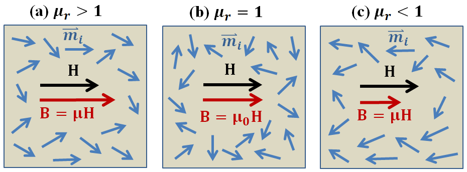
The figure above describes partial alignment of magnetic dipole moments under the influence of an inducing field for various cases.
- (a). Paramagnetic (): Dipole moment aligned parallel to the applied field and produce a net magnetization in the direction of the external field.
- (b). Non-permeable or non-magnetic ().
- (c). Diamagnetic (): Dipole moments aligned opposite to the external field, reducing the magnetic flux density.
Most rocks are paramagnetic () but some are diamagnetic () with both forms of magnetization being fairly weak. This means that they are insignificant contributors to the geomagnetic field. This is in contrast to ferromagnetic rocks, which can produce magnetic signals that are many times greater than paramagnetic or diamagnetic rocks. The strength of ferromagnetic materials comes from neighboring dipole moments interacting strongly with each other which produces a quantum mechanical effect called exchange energy. These interactions allow ferromagnetic materials to retain a magnetization even with the absence of an inducing field. This type of magnetization is called remanent magnetization or remanence.
2.7.4 Remanent magnetization
2.7.4.1 Theory for remanent magnetization
(a). Even if you take it to outer space where there is no inducing field, it is still magnetized.
(b). Ferromagnetic materials acquire remanence when they cool through its Curie temperature.
(c). Above Curie temperature, thermal energy prevents dipoles from aligning with the external field.
(d). As the materials cool down, and eventually below Curie temperature, the magnetic dipoles start to align and stay aligned.
Curie temperature
(https://en.wikipedia.org/wiki/Curie_temperature
https://www.britannica.com/science/Curie-point)
- Curie point
- Named after a French physicist, Pierre Curie, who showed that magnetism was lost at a critical temperature.
- For iron, the Curie temperature is 770
 (
( ).
). - Cobalt (
 (
( )), one of the highest Curie point.
 - Below Curie point, atoms (behave as tiny magnets) spontaneously align themselves in direction of external magnetic field (they are permanently magnetized).
- Above Curie point, materials lose their permanent magnetic properties.
As the material cools the magnetic particles can stay aligned and eventually lock into place in a domain structure. Each domain has all of its constituent dipoles locked into a single direction. This structure stays in place after the ambient field is removed and the object will have a net remanent magnetism.
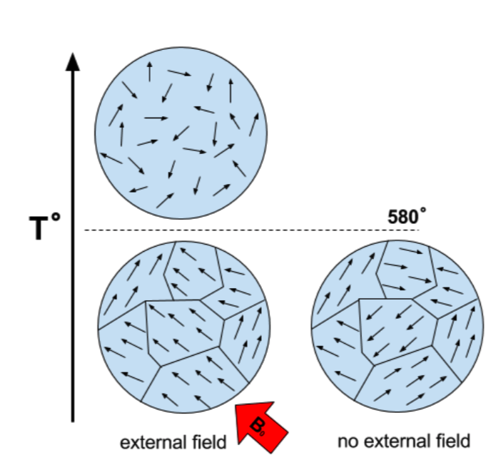
The temperature within the Earth increases with depth. We know the surface temperature, and we also know roughly how temperature increases with depth. So, a simple calculation shows that at approximately  depth, the temperature in the Earth would be higher than the Curie temperature of almost all known ferromagnetic materials.
2.7.4.2 Application for remanent magnetization
The ordnance items and other man-made objects can be detected through remanence. In the figure (b) below: these kinds of magnetic anomalies cannot be explained by induced magnetization.
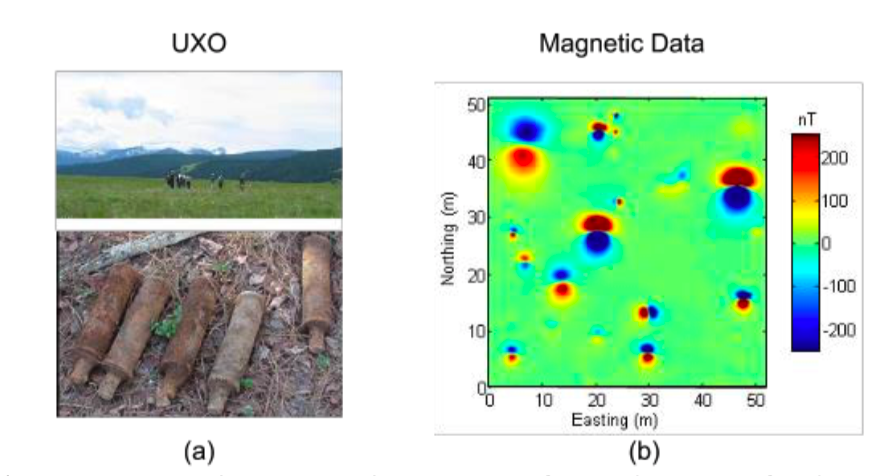
From magnetization to plate tectonics, when magnetics materials are magnetized, the magnetization direction is consistent with the direction of the external magnetic field when the magnetic materials were magnetized. Ferromagnetic materials such as basalt lava flow able to lock in a record of the direction and intensity of the magnetic field when they form (i.e., permanently magnetized). These records can be transported, rotated and faulted by plate tectonics. Therefore, these records provide information on not only the past behavior of Earth’s magnetic field and but also the past location of tectonic plates. Paleomagnetism: the study of such records in rocks, which played an instrumental role in establishing continental drift and plate tectonics as science.
On the following figure, magnetic stripping offshore Pacific Northwest, which centered around Juan de Fuca Ridge which is a mid-ocean spreading center and divergent plate boundary between Pacific plate and the Juan de Fuca plate. Magnetic striping on either side of the ridge helps data the rock and determine the spreading rate and age of the plate.
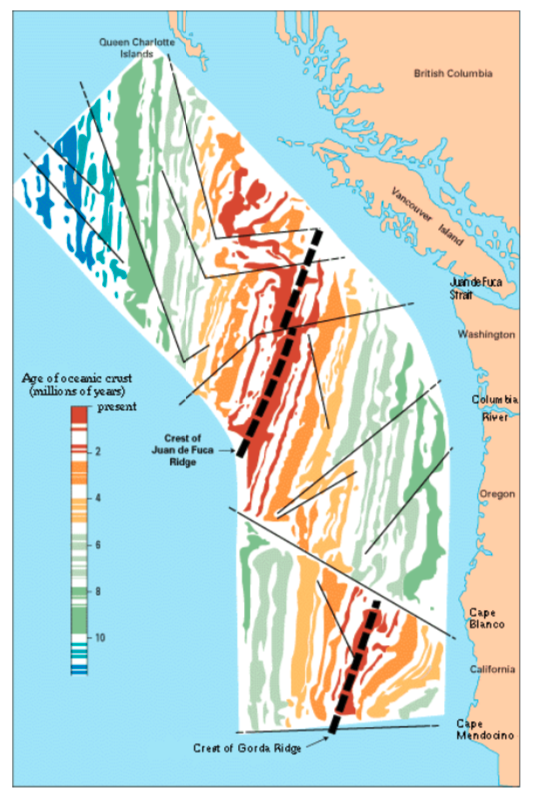
2.7.5 Total magnetization
The proper understanding is that the magnetization is composed of two parts: (a) An induced portion ( ) and (b) remanent portion (
 ). The net magnetization is:
![\[\boldsymbol M={\boldsymbol M}_{\mathbf i}+{\boldsymbol M}_{\mathbf r}\]](https://uhlibraries.pressbooks.pub/app/uploads/quicklatex/quicklatex.com-2ecdd2a2080fb1b03d40d78a397c6335_l3.png "Rendered by QuickLaTeX.com")
The relationship between magnetization  and the source
  (earth’s magnetic field) is given by:
![\[\boldsymbol M=\kappa\boldsymbol H+{\boldsymbol M}_{\mathbf r}\]](https://uhlibraries.pressbooks.pub/app/uploads/quicklatex/quicklatex.com-0cc5480472892b0a8287aa504785e19e_l3.png "Rendered by QuickLaTeX.com")
where is the magnetic susceptibility.
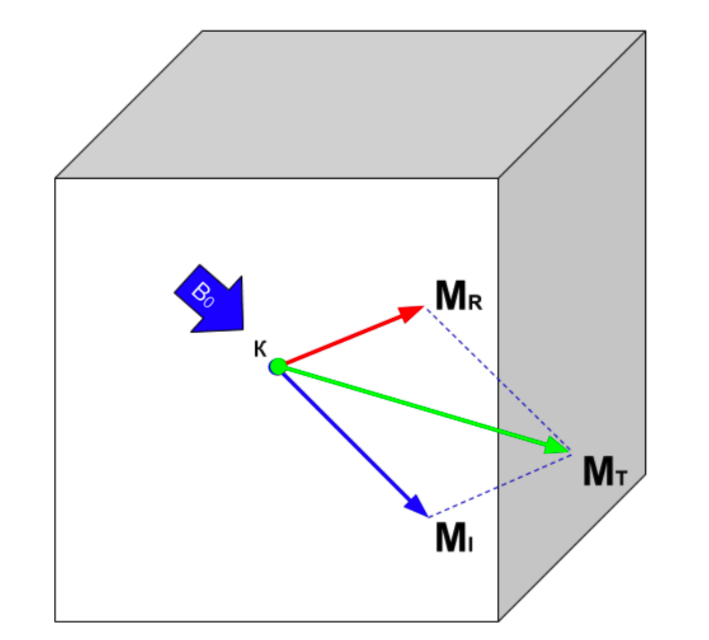
The composite field is below:
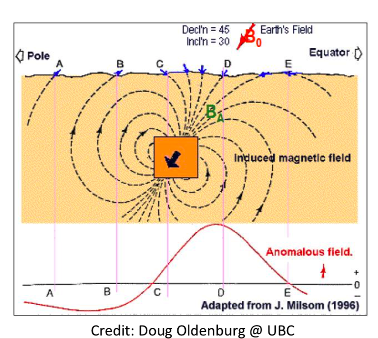
Composite field:
![\[\boldsymbol B={\boldsymbol B}_{\mathbf 0}+{\boldsymbol B}_{\mathbf A}\]](https://uhlibraries.pressbooks.pub/app/uploads/quicklatex/quicklatex.com-b64917fd07143d87b5e8363ce9ad9554_l3.png "Rendered by QuickLaTeX.com")
where  is a vector,
Total field:
![\[\left|\boldsymbol B\right|=\left|{\boldsymbol B}_{\mathbf 0}+{\boldsymbol B}_{\mathbf A}\right|\]](https://uhlibraries.pressbooks.pub/app/uploads/quicklatex/quicklatex.com-c8b0fa75fc96df40b3e86f70f69cc3d6_l3.png "Rendered by QuickLaTeX.com")
Majority of instrumentation measures  , i.e., total magnetic intensity, or TMI. Newer platforms can acquire three-component magnetic field. Latest instrumentation measures magnetics tensor.
Measured field: 
The total field anomaly: 
if  , then that is , total field anomaly
  is the projection of the anomalous field onto the direction of the inducing field.
![\[\triangle\overrightarrow B\simeq\triangle\overrightarrow{B_A}\cdot{\widehat B}_0\]](https://uhlibraries.pressbooks.pub/app/uploads/quicklatex/quicklatex.com-9612638bb08c1186ba03acda567b6367_l3.png "Rendered by QuickLaTeX.com")
Tips for ploting magnetic anomalous field
- First, find the location with zero field (C and E location above the figure).
- Second, decide
 direction and calculate the projection of to
  .
.
-
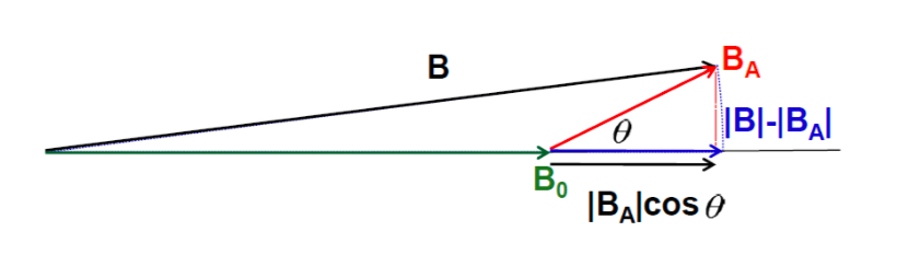
Credit: Doug Oldenburg @ UBC
A wrong example
Something is wrong!!!
The magnetic anomaly field is not zero at C location. It should be a small positive value.