4.1 data enhancement

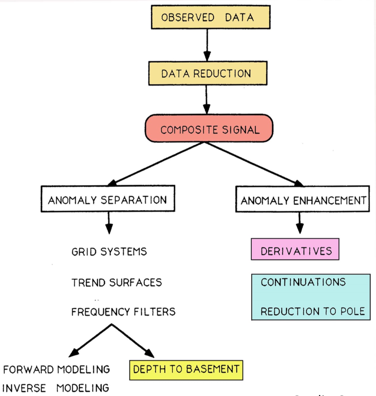
In previous chapters, we have discussed a lot about processing data which contains contributions from many sources, these sources have different physical properties and different scales or depths. Specifically, we have focused on anomaly separation from the observed data to remove unwanted contributions and single out the signal from targets. In practice, we would also apply various anomaly enhancement methods, in order to increase the visibility, or interpretability, or importance of the desired features, or signals with respect to others. Anomaly enhancement does not remove unwanted signals, instead, it helps to diminish or suppress their manifestation on a data map. There are many enhancement methods, such as the histogram equalization technique, and various types of derivative-based enhancement methods. We will discuss them in detail in this chapter.

4.1.1 Histogram equalization technique

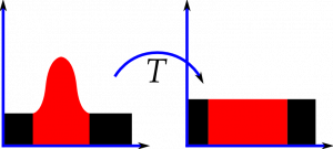
Histogram equalization technique is a common method in image processing to increase contrast in the intensities, such as in the pixel values intensity so that the adjusted values can be better distributed on the histogram, as illustrated in the image below.

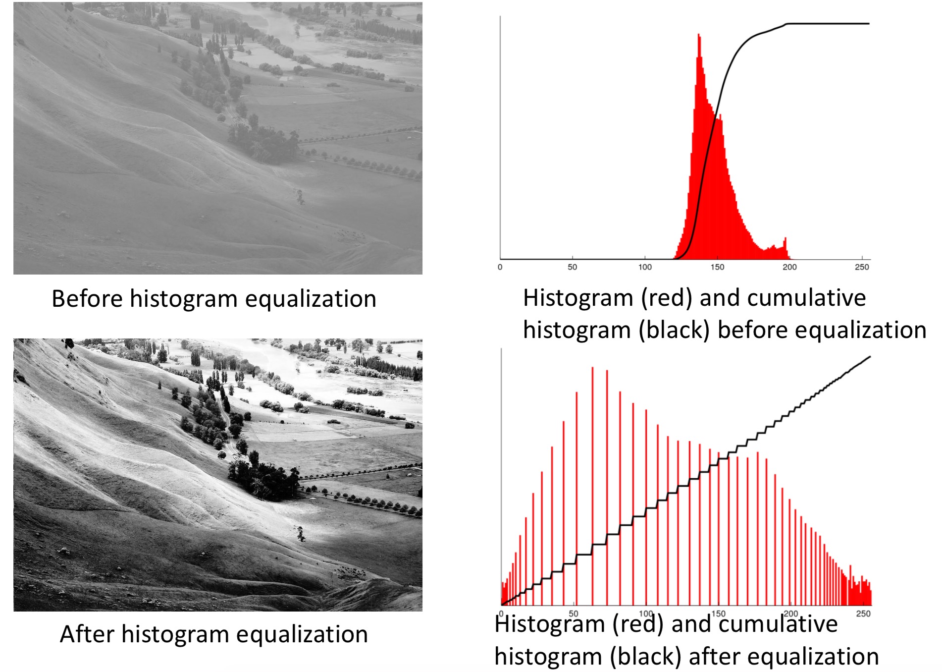
The technique allows for areas of lower local contrast to gain a higher contrast, through spreading out the most frequent intensity values in the histogram. In the example of the figure shown below, the top row displays the original image and its pixel values histogram (in red) and its cumulative histogram (in black) before applying the histogram equalization method; The image is blurry, and the pixels values are concentrated within a narrow range. However, after implementing the equalization (shown in the bottom row), the pixel values are spread out in a wider range, and the resulting image is sharper and therefore more details could be visualized.

Application to geophysics

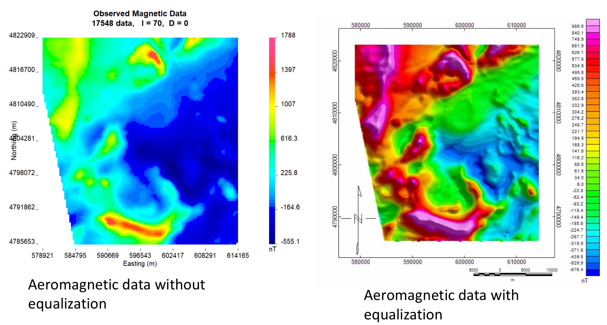
In geophysical data, subtle features in data images with a high dynamic range, such as aeromagnetic data, are difficult to be visualized. Histogram equalization can help to bring out these subtle features. For example, the left figure below is the observed aeromagnetic data image without equalization, while the right figure displays the data after equalization was applied; We can observe that large-amplitude features are still there, while the smaller amplitude values (around 0) which are not clearly shown in the original figure now become more clearly visible to our naked eyes.

4.1.2 Derivative-based enhancement methods

Usually, the anomalies to be enhanced are of small spatial scales than that of those we want to suppress. In general, features with shorter wavelengths are associated with steeper gradient and greater curvatures. Therefore, derivative-based methods are among the most widely used techniques for enhancing anomalies.

There are many derivative-based methods, such as the vertical derivative, total horizontal derivative, tilt derivative, and total horizontal derivative of the tilt derivative, which we will discuss in the following. Other enhancement methods are also popular, such as downward continuation, strike filtering, and phase preserving dynamic range compression filter (https://www.peterkovesi.com/projects/tonemapping/index.html).

4.1.2.1 Vertical derivative

The vertical derivative of the data image could enhance the visibility and interpretability of the original data image.

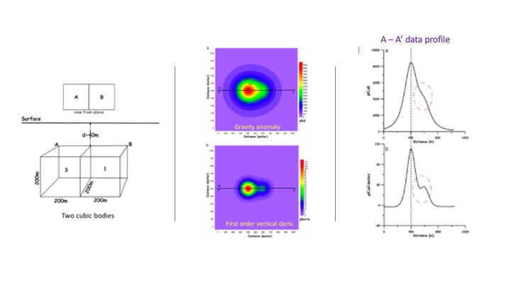
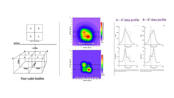
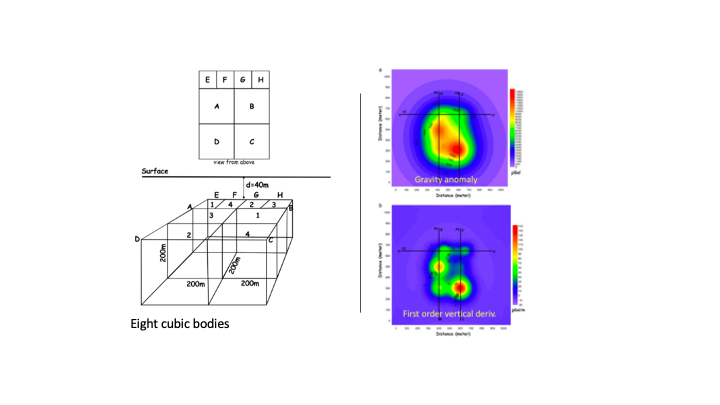
For example, as shown in the synthetic modeling figures below, the gravity gradient image () is compared with the gravity anomaly image () in several synthetic models, with a different number of anomaly blocks in the subsurface. Generally, in comparison with the gravity images, the vertical derivative images could be used to better define and differentiate the spatial locations of the blocks, and more accurately to determine the number of blocks from the data images, while the gravity anomaly images cannot be used to clearly separate the signals from multiple blocks.

4.1.2.2 Total horizontal derivative

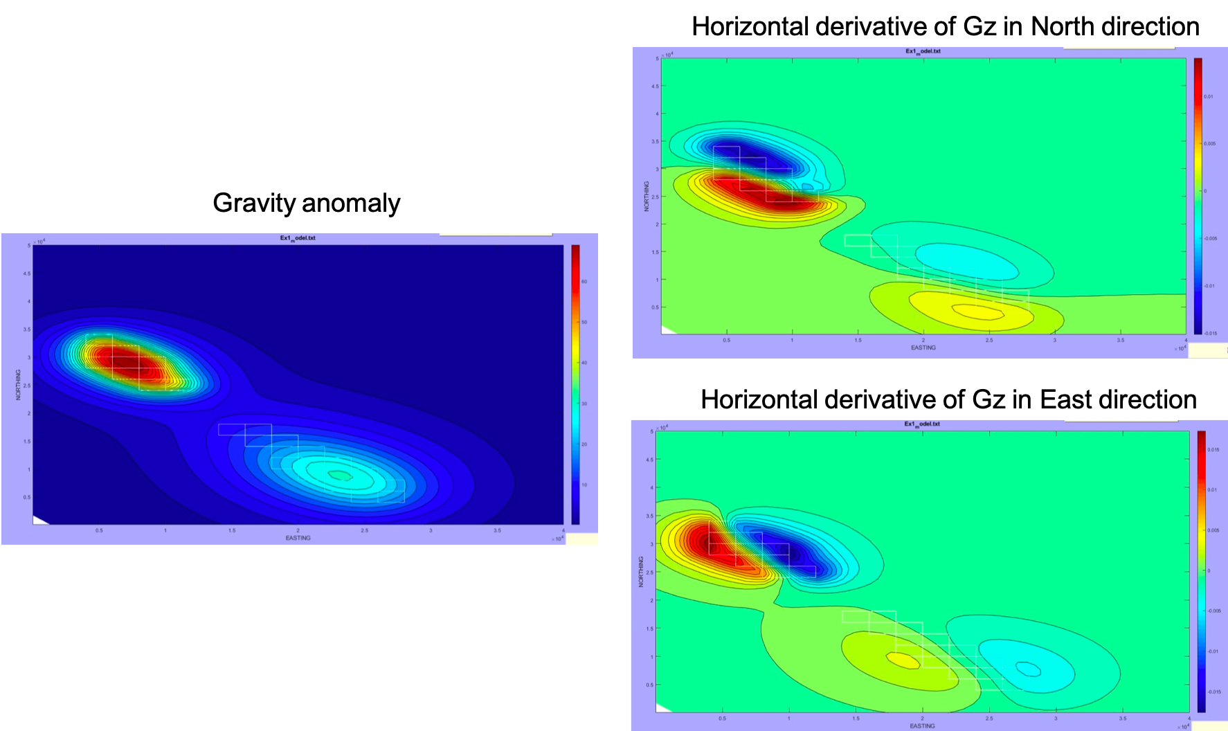
Similar to the vertical derivative of the data, the horizontal derivative of the data image could also be used to better enhance the anomaly interpretability.

For example, the figures below represent the gravity data , the horizontal derivative of in the North direction, and horizontal derivative of in the East direction, respectively. All the derivative data images can be used to better define the boundaries of the target features in the subsurface. More specifically, the horizontal derivative in the North direction defines the north/south boundary of the target body, while the horizontal derivative in the East direction defines the west/east boundary of the target body. Altogether, the derivative images could help us determine the general boundary of the target feature.

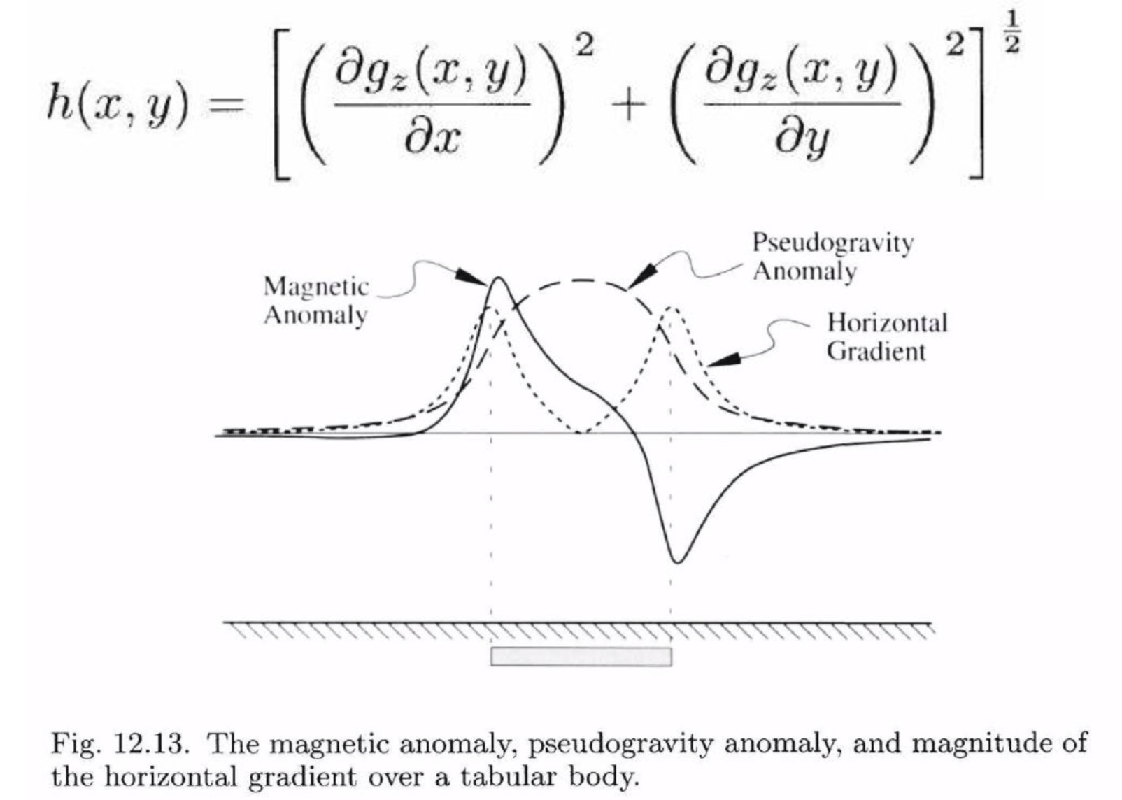
The total horizontal derivative magnitude is the square root of the sum of the squares of the horizontal derivatives in (or E/W) and (or N/S) directions. Its math expression and an example are shown in the following.

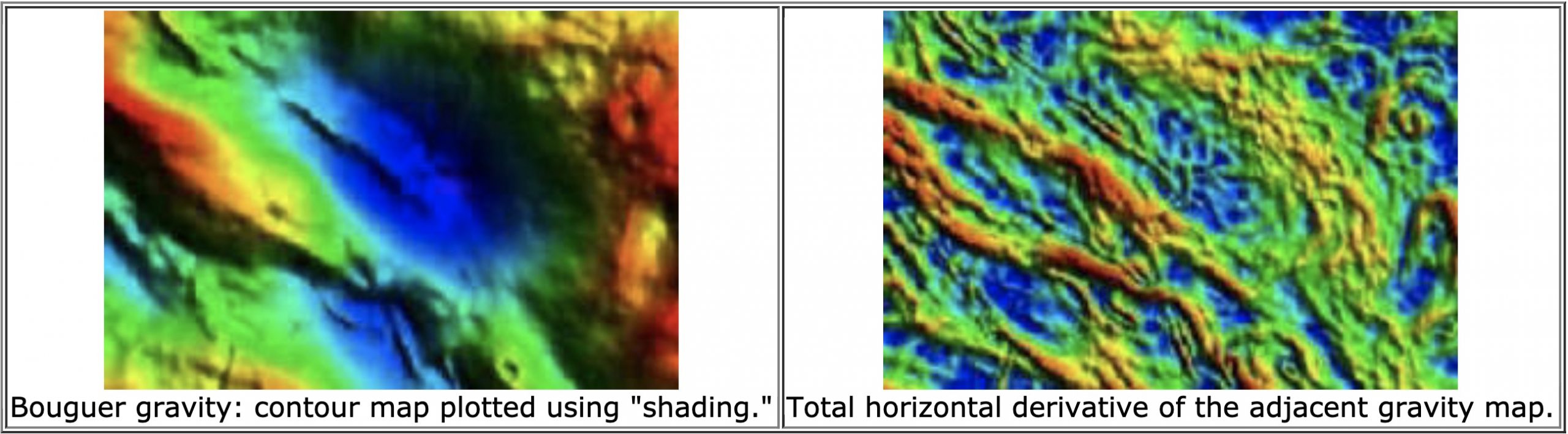
Another comparison example was shown in the images below, the total horizontal derivative of the gravity data shows much more detailed structures in comparison to the Bouguer gravity map.

4.1.2.3 Tilt derivative

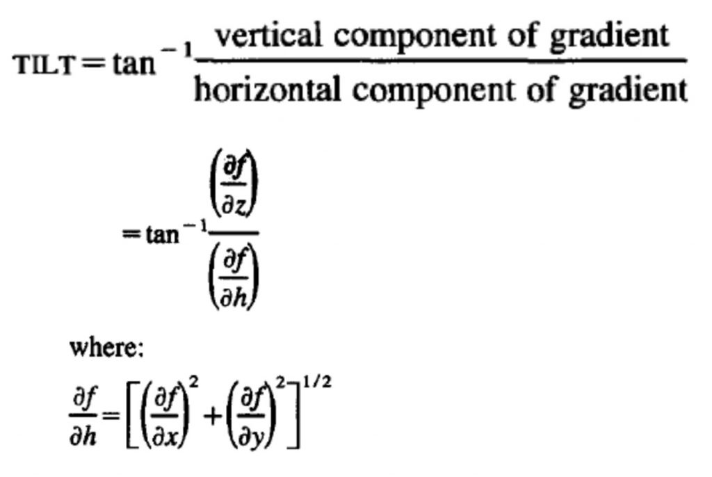
Tile derivative is the arctangent of the ratio between the vertical derivative and the total horizontal derivative of the data. Its mathematical expression is shown in the following.

We can compare and contrast the characteristics of different derivatives of the data along with the tilt derivative of the gravity data simulated from two density blocks buried at different depths shown below.

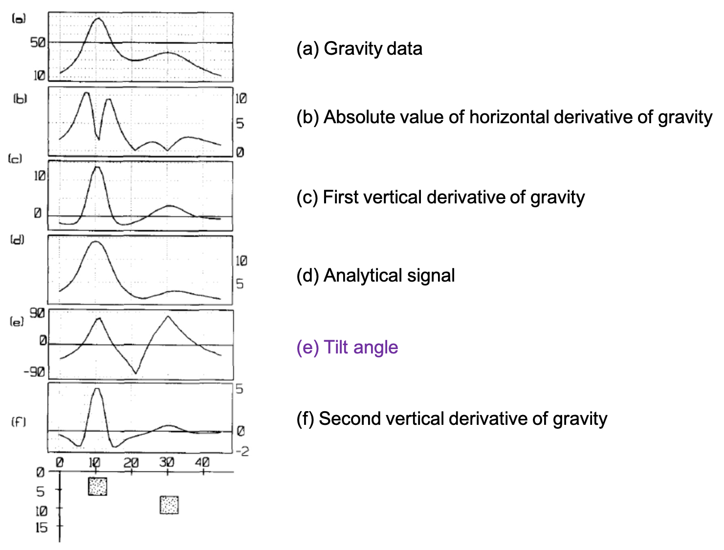
Based on the data images above, we can make the following observations:

• in figure (b), the horizontal derivative shows 2 peaks corresponds to the boundary of the blocks;
• in figure (c), the vertical derivative shows a more compact pattern, which defines the shape and distribution of the source bodies;
• in figure (e), the tilt angle image shows two signal peaks, where the peak from the deeper body is comparable in amplitude with the shallower body signal peak! And the peaks are right above the body locations. That is the significant characteristic of the tilt angle enhancement method.

If we further take the horizontal derivative of the tilt angle, then the data profile will show the boundary of the source bodies, and this will be called the horizontal derivative of the tilt derivative.