Chapter 7: Inversion

Jiajia Sun

7 Chapter 7: Inversion

7.1 Inversion: basic theory

7.1.1 A simple example

Let’s consider a physical system with two objects, with unknown masses of $m1$ and $m2$ , respectively. The first data measurement is the weight of the first object, which is 1 kg; And our second data is the weight of the second object, which is 2 kg; Our third data is the combined weight of the two objects, which is 2 kg. Thus, for this particular experiment, we have 3 data measurements with 2 unknowns.

The above statements can be mathematically expressed as the following data equations with the measurement errors considered:

$1={{d}_{1}}={{m}_{1}}+{{\varepsilon }_{1}}$

$2={{d}_{2}}={{m}_{2}}+{{\varepsilon }_{2}}$

$2={{d}_{3}}={{m}_{1}}+{{m}_{2}}+{{\varepsilon }_{3}}$

From these data equations, we can observe that they are not consistent with each other due to the existence of the measurement errors. However, there is no reason to discard one of the three equations in favor of the other two, since we don’t know which data equation is more contaminated by the measurement error. Therefore, we need to use all the data samples we have.

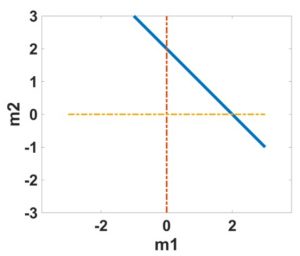
Now let’s try to understand these data equations graphically. As shown from the graph, the three lines do not intersect at a single point, which indicates that the equations are inconsistent with each other. Our problem is, based on the three data measurements, where is our solution of $m1$ and $m2$ ?

Image credit: ROEL SNIEDER and JEANNOT TRAMPERT

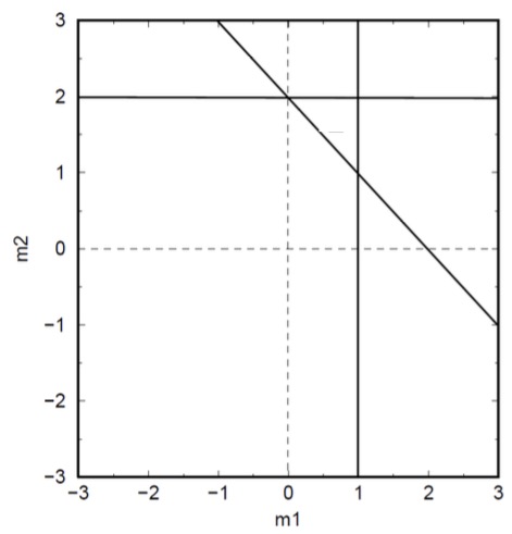
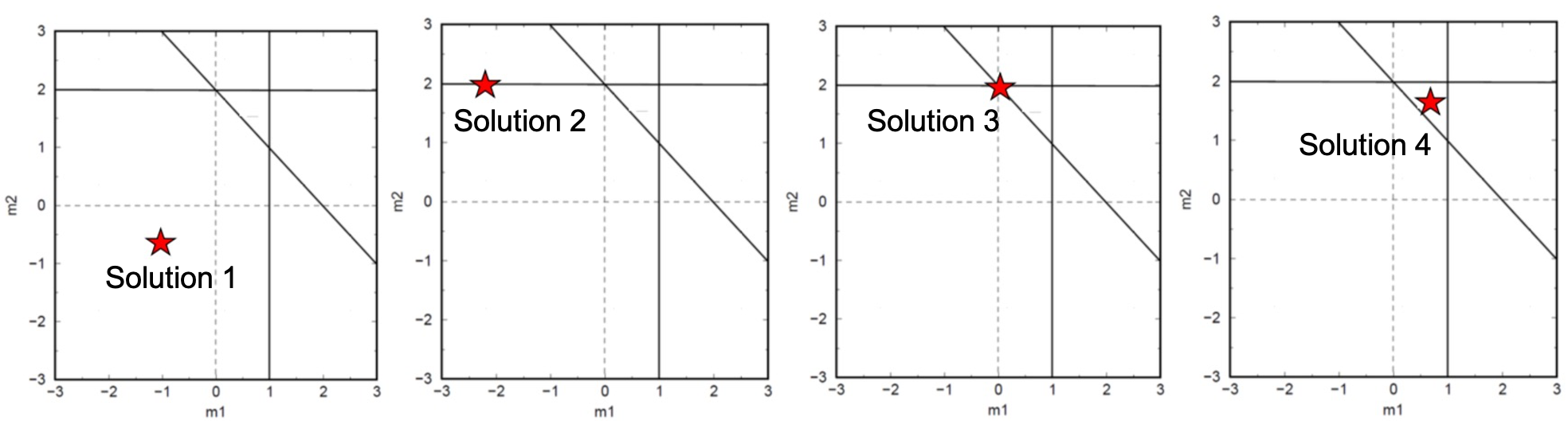
If the red star shown in the graph represents the possible solution, at position 1, it is a poor solution since it didn’t satisfy any of the three data equations; at position 2, it is a better solution since it satisfies one of the data equations; at position 3, it’s an even better solution since it satisfies two of the data equations. At position 4, this solution doesn’t satisfy any of the data equations, but on average it has a minimum distance to all three lines. Thus, this approximate solution seems to be better than other solutions, since it represents the best compromise and gives the best fit to the data.

In order to find a solution, we need to do some math. Firstly, we can re-write the above data equations into a more compact matrix and vector form, which is as follows:

$\vec{d}=\mathbf{A}\vec{m}+\varepsilon$

Where we defined the data measurements into the vector $\vec{d}$ , unknowns as vector $\vec{m}$ , errors as vector $\varepsilon$ , a matrix $\mathbf{A}$ , which is coefficients:

$\vec{d}=\left[ \begin{matrix} 1 \\ 2 \\ 2 \\ \end{matrix} \right]$

$\vec{m}=\left[ \begin{matrix} {{m}_{1}} \\ {{m}_{2}} \\ \end{matrix} \right],\vec{\varepsilon }=\left[ \begin{matrix} {{\varepsilon }_{1}} \\ {{\varepsilon }_{2}} \\ \end{matrix} \right]$

$\mathbf{A}=\left[ \begin{matrix} 1 & 0 \\ 0 & 1 \\ 1 & 1 \\ \end{matrix} \right]$

To summarize, using the three measures $\vec{d}$ we have, we want to find a model $\vec{m}$ that minimizes the difference between measured data $\vec{d}$ and predicted data $\mathbf{A}\vec{m}$ . Therefore, we need to first define this difference, then minimize it. The math expression of this difference can be defined by using the L2 norm as follows:

$\text{minimize: }\phi \left( m \right)=\left\| d-\mathbf{A}m \right\|_{2}^{2}$

This is called the objective function, or cost function.

Now, the problem becomes how to minimize this objective function. This can be easily done by setting the derivative of $\phi \left( m \right)$ with respect to $m$ to 0. By using matrix calculus, the derivation is as follows:

$\frac{\partial \phi }{\partial m}=2-{{\mathbf{A}}^{T}}\left( d-\mathbf{A}m \right)=0$

${{\mathbf{A}}^{T}}\mathbf{A}m={{\mathbf{A}}^{T}}d$

$m={{\left( {{\mathbf{A}}^{T}}\mathbf{A} \right)}^{-1}}{{\mathbf{A}}^{T}}d$

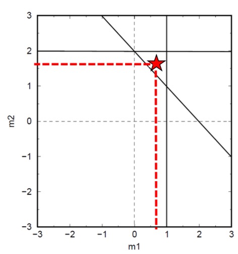
Therefore, by substituting above solution formula, the solution to our problem is as follows:

$m=\left[ \begin{matrix} {}^{2}\!\!\diagup\!\!{}_{3}\; \\ {}^{5}\!\!\diagup\!\!{}_{3}\; \\ \end{matrix} \right]$

The graphical representation of this solution is shown as the red star in the graph below.

A quick summary up to here: we have used the weight data measurements to estimate the mass of each object. This is actually inversion!

7.1.2 Inversion

Inversion is all about estimating parameter values based on some measurements. Inversion is ubiquitous in every physical discipline, such as geophysics, medical imaging, astrophysics, etc. Sometimes inversion is also called model parameter estimation. The parameters we are trying to estimate will help us to understand a physical system. For example, in geophysics, the physical system we are trying to understand is Earth or a particular study area on Earth.

There are many detailed books and resources, out of many resources, there are three books we strongly recommend. One is the Parameter Estimation and Inverse Problems by Richard C. Aster et al. (https://www.sciencedirect.com/book/9 780123850485/parameter-estimation- and-inverse-problems), and Geophysical Data Analysis: Discrete Inverse Theory (MATLAB Edition) by William Menke (https://www.sciencedirect.com/book/ 9780123971609/geophysical-data- analysis-discrete-inverse-theory), and Inverse Problem Theory by Albert Tarantola (http://www.ipgp.fr/~tarantola/Files/ Professional/Books/InverseProblemTheory.pdf). Inversion for applied geophysics: a tutorial written by Douglas Oldenburg and Yaoguo Li (2005) is also very helpful.

7.1.3 Least-squares solution

Back to what we have talked so far, from the data equation in the matrix-vector format as follows:

$\vec{d}=\mathbf{A}\vec{m}+\varepsilon$

The solution we obtained is from minimizing the objective function of

$\text{minimize: }\phi \left( m \right)=\left\| d-\mathbf{A}m \right\|_{2}^{2}$

This solution is called the least-squares solution in literature. In particular, the least-squares solution is applied when we have more data than unknows parameters and assumed that data have errors.

7.1.4 Minimum norm solution

Another concept is called the minimum norm solution. In order to understand this, let’s consider another simple example.

Assume we have two objects with unknown masses, $m1$ and $m2$ . Suppose the combined weight of them is measured to be 2 kg, assuming no data errors involved. Then we can formulate the data equation as follows:

$2={{d}_{1}}={{m}_{1}}+{{m}_{2}}$

Where we have 1 data, 2 unknown model parameters. i.e., less data, more parameters.

Our inverse problem is that, given this 1 data, what are the values of $m1$ and $m2$ ?

The graphical representation of this data equation (denoted as the blue line) as shown in the graph below.

We can simply observe that any point (denoted as the red star) lies on this blue line is a solution to this inverse problem. That is, there are infinite solutions.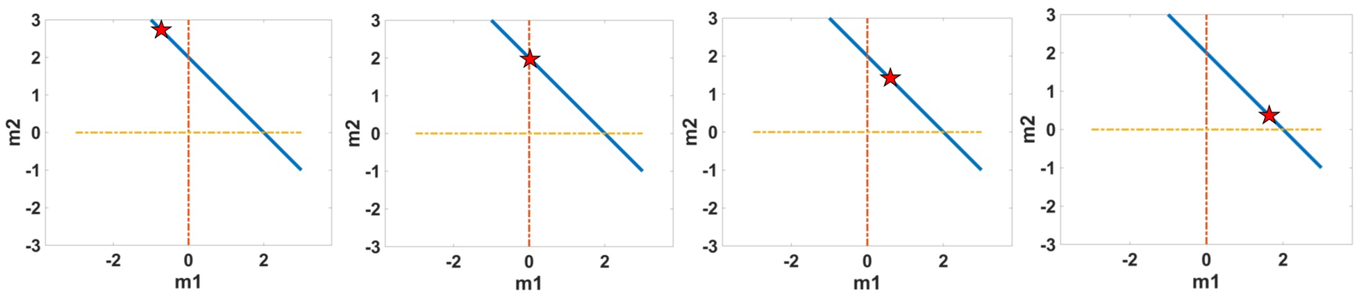

However, of all the solutions, we are interested in one solution that has the minimum norm (i.e., the shortest distance to the origin), since philosophically, people found that the minimum norm solution makes the most geological sense.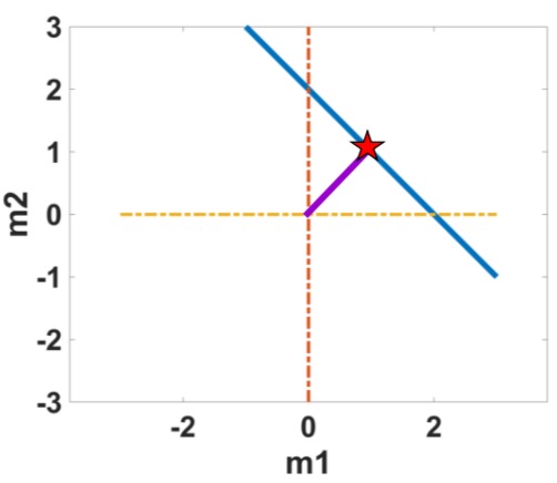

Mathematically, we are interested in the solution:

$\text{minimize: }\left\| m \right\|_{2}^{2}$

$\text{subject to: }d=\mathbf{A}m$

The minimum norm solution derivations are as follows:

$\text{minimize }\phi \left( m \right)=\left\| m \right\|_{2}^{2}+{{\lambda }^{T}}\left( d-Am \right)$

$\frac{\partial \phi \left( m \right)}{\partial m}=2m-{{A}^{T}}\lambda =0$

$m=-\frac{1}{2}{{A}^{T}}\lambda$

$\text{substitute }m\text{ back to }d=Am:$

$d=A\left( -\frac{1}{2}{{A}^{T}}\lambda \right)=-\frac{1}{2}A{{A}^{T}}\lambda$

$\lambda =-2{{\left( A{{A}^{T}} \right)}^{-1}}d$

$\text{substitute }\lambda \text{ back to }m=-\frac{1}{2}{{A}^{T}}\lambda :$

$m=-\frac{1}{2}{{A}^{T}}\left( -2{{\left( A{{A}^{T}} \right)}^{-1}}d \right)={{A}^{T}}{{\left( A{{A}^{T}} \right)}^{-1}}d$

For our example, substituting data vector and A matrix into the minimum norm solution formula, we will have the following result:

$\vec{d}=\left[ \begin{matrix} 1 \\ \end{matrix} \right]$
$A=\left[ \begin{matrix} 1 & 1 \\ \end{matrix} \right]$
$\vec{m}=\left[ \begin{matrix} 1 \\ 1 \\ \end{matrix} \right]$

A quick summary:

In the first example, we have more data than unknowns, and data contains error. The problem is called over-determined problem, the least-squares solution is
- $m={{\left( {{\mathbf{A}}^{T}}\mathbf{A} \right)}^{-1}}{{\mathbf{A}}^{T}}d$
n the second example, we have less data than unknowns, and assuming data have no errors. This type of problem is called under-determined problem, the minimum norm solution is
- $m={{A}^{T}}{{\left( A{{A}^{T}} \right)}^{-1}}d$

Potential field data inversions are mostly under-determined problems. For example, in an airborne magnetic study, there are less than 2000 data, but there are about 2.6 million unknown susceptibility model parameters.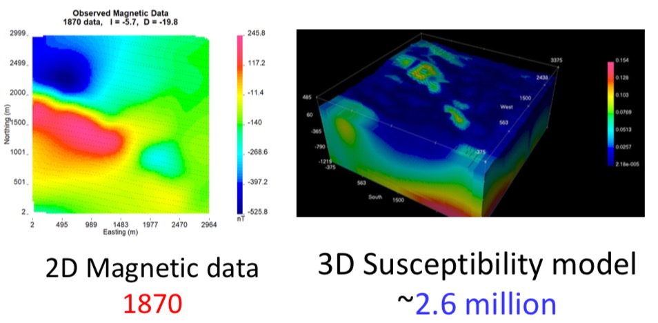

7.1.5. Under-determined inverse problems

An inverse problem is under-determined when the number of data types is less than the number of unknown parameters. This is a common situation with potential field data inversion, where most of the problems are under-determined in nature. Normally, we would solve inverse problems using the following equation:

$\~m = A^T(AA^T)^{-1}d$

Unfortunately, this equation cannot be used directly to solve under-determined inverse problems as the term $AA^T$ is ill-conditioned, which we will explain below.

Take the following equation for linear inverse problems:

$A\vec{m} = \vec{d}$

The matrix $A$ has a property that we can describe as the condition number. The condition number measures how much our model $\vec{m}$ would change for a small change in the data term $\vec{d}$ . This is highly relevant in inverse problems as all geophysical field measurements will have errors, and we do not want these errors to overly influence our inverse solutions. We can describe the condition number as the ratio of relative error in the solution to the ration of relative error in the data. Mathematically, we can describe the condition number using the following equation:

$cond(A) = max[\frac{||A^-1e||}{||e||}\frac{||d||}{||A^-1d||}] = ||A^{-1}|| ||A||$

where $||*||$ represents a matrix norm, d represents clean data, and e represents data errors from noisy data subtracted by clean data.

From the equation above, we can come to the conclusion that if the condition number of an inverse problem is large, than a tiny change such as measurement errors would create a huge change in the inverse solution. When this is the case, we can state that the inverse solution is unstable, and the inverse problem ill-conditioned. In order to calculate the condition number, we can simply use singular value decomposition (SVD).

7.1.6. Ill-conditioned problems

Unfortunately, most geophysics inversion problems are ill-conditioned. This means that the problems have a large condition number $cond(A)$ . Normally, we would solve inverse problems using the following two equations: $\~{m} = (A^TA)^{-1}(A^Td)$ and $\~{m} = A^T(AA^T)^{-1}d$ . However, the large size of $cond(A)$ also means that $cond(A^TA)$ would also be large, which prevents us from directly using the prior equations to find an inverse solution.

Before we can find a solution to ill-conditioned problems, we first must discuss the terms ill-posed and well-posed in the context of an inverse problem. A problem is well-posed when it has a solution, the solution is unique, and the solution is stable. If a problem does not meet all of these three criteria, it is instead ill-posed. Inverse problems are often ill-posed, as an inverse solution may not exist (over-determined), the solution may be non-unique (under-determined), or the solution may be unstable (ill-conditioned). In the case of ill-conditioned problems, the instability of the inverse solution is caused by a large condition number. This also means that reducing the condition number would increase the stability of the solution. The simplest way to reduce the condition number is by adding a small positive value to the diagonals of matrix A.

As an example, we will use the following matrix A:

$\begin{matrix} 3.0000&7.0000\\ 1.5000&3.5001 \end{matrix}$

We can use programming languages such as MATLAB to solve for the condition number of A, resulting in $cond(A) = 2.4167e+05$ . This is a remarkably large value, and we can use a smaller matrix b $\begin{matrix} 3.0000\\ 1.5000 \end{matrix}$ to observe the factors that contribute to the condition number. Finding the inverse solution of matrix A and matrix b $A \backslash b$ results in a simple solution of $\begin{matrix} 1\\ 0 \end{matrix}$ . However, adding a small value such as $0.01$ to matrix b forms matrix c: $\begin{matrix} 3.0100\\ 1.5100 \end{matrix}$ which has a vastly different inverse solution $A \backslash c$ : $\begin{matrix}-1.1657e3\\ 0.5000e3 \end{matrix}$ . This shows that small changes in measurements can result huge changes in the inverse solution, as A is ill-conditioned.

Now, we will show the difference that adding a small positive value such as $0.1$ to the diagonals makes to solving matrix A:

$\begin{matrix} 3.1000&7.0000\\ 1.5000&3.6001 \end{matrix}$

The condition number of the modified matrix is now only $cond(A) = 111.7881$ , which is orders of magnitude smaller than our previous result. Additionally, our inverse solutions using matrices b and c now result in the following solutions: $A \backslash b = \begin{matrix} 0.4548\\ 0.2272 \end{matrix}$ and $A \backslash c = \begin{matrix} 0.4033\\ 0.2514 \end{matrix}$ . By adding the small positive value, matrix A is now well-posed.

7.1.7. Regularization

Dealing with an ill-conditioned inverse problem through methods such as adding a small positive value to the diagonals is called regularization. We can represent one form of regularized inversion using the Levenberg-Marquardt algorithm:

$\~{m} = (A^TA + \lambda I)^{-1}(A^Td)$

$\~{m} = A^T(AA^T + \lambda I)^{-1}d$

Interestingly, these two equations can also now be proved to be exactly equal. This representation of regularized inversion is called the damped least-squares solution, and can also be called the regularized least-squares solution. The equation $\~{m} = (A^TA + \lambda I)^{-1}(A^Td)$ can be considered to be the solution to an inverse problem, so instead we will take a look at the following expression to gain a better understanding of what damping (or regularization) does:

Minimize:

$\phi(m) = ||d - Am||^2_2 + \lambda||m||^2_2$

The first term: $||d - Am||^2_2$ tries to find a model that gives the best fit to the data provided. This is called the data misfit term. The second term: $\lambda||m||^2_2$ tries to find a model with the smallest normalization, and is called the regularization term. Unfortunately, both terms cannot be minimized at the same time, so the parameter $\lambda$ controls the trade-off between the two conflicting objectives. There are more ways of implementing regularization and many different regularization terms, but $||m||^2_2$ is the simplest one.

7.2 Inversion: Potential field data

7.2.1. inverse problem

Currently, the relationship between geophysical modal and data can be expressed below:

$F\left[\textbf{m}\right]+\varepsilon\;=\;\textbf{d}$

where, $F$ is forward mapping operator. $\textbf{m}$ is Earth model, e.g., density model, velocity model, which is unknown in inversion. $\varepsilon$ is errors from observation, discretization or assumptions and $\textbf{d}$ is observed data from geophysical survey. Here we note that $\textbf{d}$ here is clean data.

Overly speaking, inverse solution can be regarded as a mathematical process that we need to find a plausible model given observed data, estimated errors and a forward modeling method. During inversion, we need to solve two problems: forward problem and inverse problem.

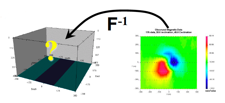
The forward problem plays critical role during inversion. Here is an example about magnetic data and susceptibility model to illustrate how the forward problems work. Compared with inversion, forward modeling means we can calculate the data given a model (seeing figure below).

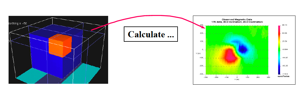
Mathematical expression of calculating magnetic data based on the susceptibility model is shown below:

$b_i=\sum_{j=1}^MG_{ij}\kappa_j$

or

$\overset\rightharpoonup b=\textbf{G}\overset\rightharpoonup\kappa$

where $b_i$ ( $i=1, N$ ) is calculated data and $\kappa_j$ ( $j=1, M$ ) is a given susceptibility distribution.

The basic understanding of inverse problem is shown carton below:

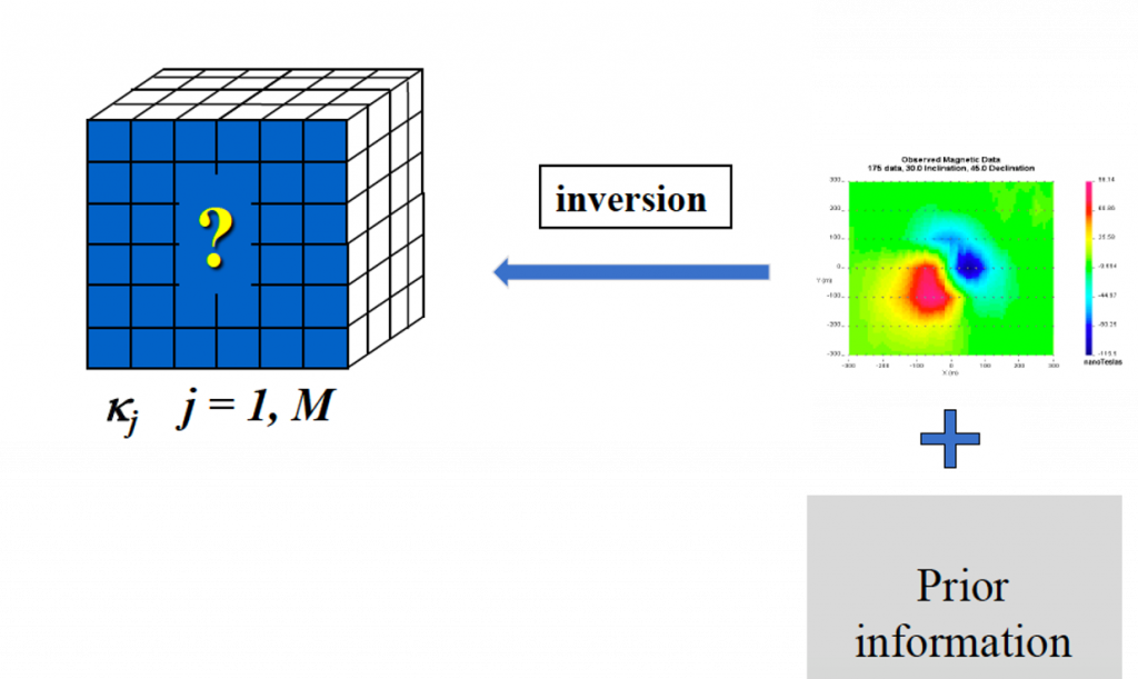
Basic understanding of inverse problems.

The figure above shows that given an observed geophysical data incorporated some prior information, we need to estimate a reasonable model that can reproduce the observed data well. The reason we need to incorporate prior information is that the potential field data always associated with non-uniqueness problem. Non-uniqueness problem will be introduced in following section.

Summary of inversion

Given: data, error, a forward modeling and prior information about geology.

Find: a plausible model that could generate the geophysical data and is consistent with known geologic information.

Objective: produce a model that helps better understand geology.

7.2.2. non-uniqueness

7.2.2.1. Basic concepts about the non-uniqueness problem

Inversion can be taken as an optimization problem, the mathematical equation is following:

$\phi(m)=\left\|d-Am\right\|_2^2+\lambda\left\|m\right\|_2^2$

Look at the right hand side of the equation above, the first term is named data misfit term related the error between predicted data and observed data. The second is regularization term measuring the spatial correlation which is also helpful to reduce the non-uniqueness problem during inversion.

There are three aspects about the non-uniqueness:

(1). Number of data is smaller than number of unknown parameters which is termed under-determined problem.

(2). Data have errors.

(3). Inherent ambiguity associated with potential field data.

In the first aspect, inversions using potential field data is an under-determined problem that means there are existence of infinite solutions, where each solution can reproduce observed data equally well. Thus, the non-uniqueness arises from the infinite solutions. The data errors and inherent ambiguity also affect non-uniqueness problem and these two parts will be specifically talked in the following two sections.

7.2.2.2. Data errors

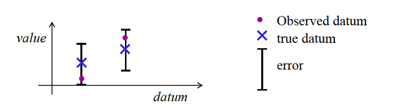
Data errors commonly and widely exist during geophysical measurements. Understanding errors and the meaning of fitting data are significant during inversions. Here is an example, in the figure below, the red circles represent the measured data with the noise that also means each red circle has errors. Blue curve is the simulated data from the particular models shown in the bottom figure. In geophysical inversion, we need to fit the measured data (red circle). Observations from the top figure, most simulated data (blue curve) fit the measured data (red circle) well. But we also noticed some bad fitted points because of the noise during the measurements. So in this scenario, It is important to consider what the meaning of “fitting” the data, especially when the data are inaccurate.

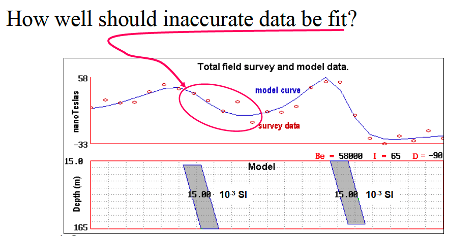
Data fitting map. (Credit: Yaoguo Li @ CSM)

In the following contents, we will explore the basic concepts about noise and data misfit. The figure below shows that if observations are inaccurate, we should not to perfectly fit the observed data. The reason is the noise will be propagated to the inverted models when we perfectly fit the noised data. Thus, we can obtain a basic principle during inversion that the model produced by inversion must NOT fit data exactly.

Observed data, true data and error. (Credit: Yaoguo Li @ CSM)

7.2.2.3. Inherent ambiguity

Before talking about inherent ambiguity, let us recall the first identity (the more details, please refer slides 19 from lecture4 or the chapter 2 in this book).

First identity

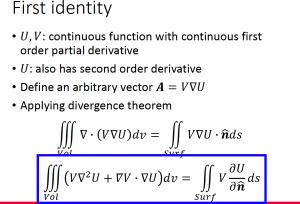
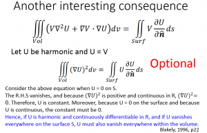
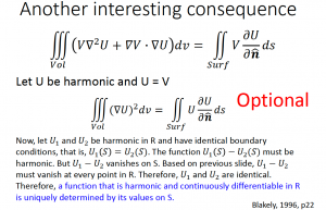
Base on the first identity, we can obtain several implications for equivalent source.

A function that is harmonic and continuously differentiable (e.g., gravity data and magnetic data) in R is uniquely determined by its values on S.
Gravity and magnetic scalar potentials are harmonic and continuously differentiable.
Therefore, gravity and magnetic scalar potentials are uniquely determined by their values on S.
Therefore, gravity and magnetic data are uniquely determined by their values on S.

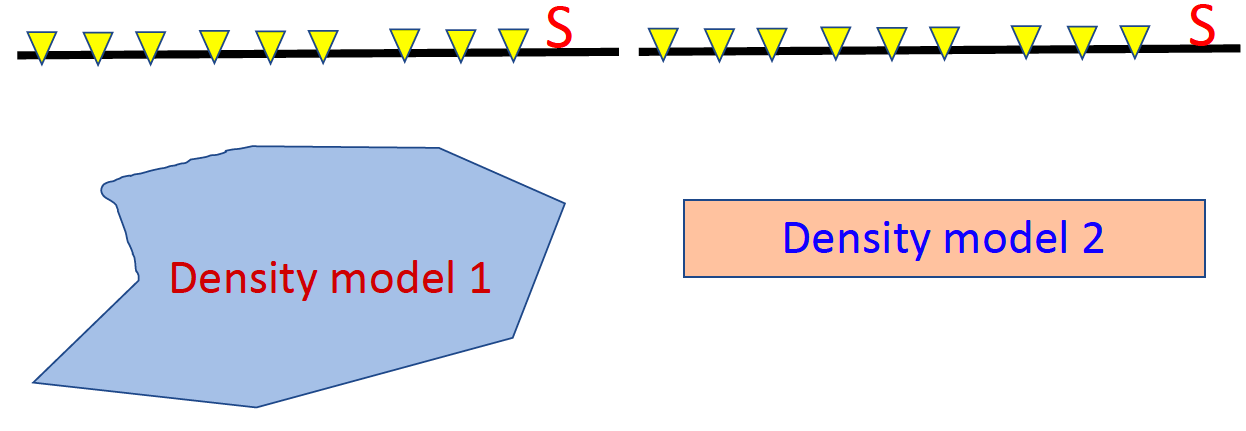
How to understand equivalent source? Here is an example, assuming the gravity measurements, calculated from density model 1 and density model 2, are exactly same. The gravity fields above the surface are same as well, which means if the measurements on S are the sam, then the gravity data in R from these two density models are the same. These two sources are called equivalent source.

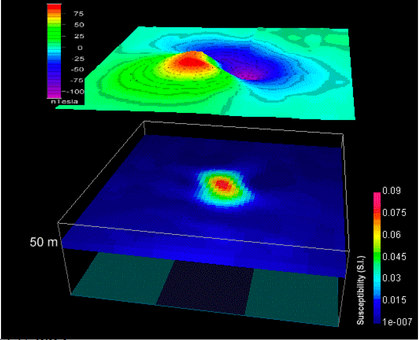
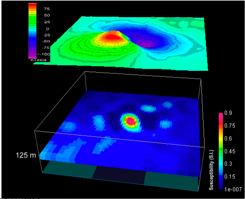
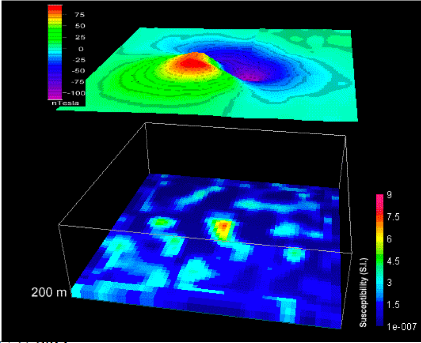
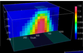
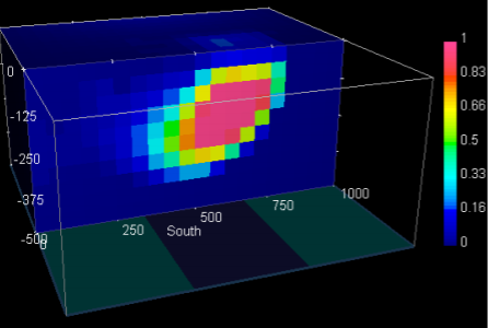
Another example is below. Assuming we have a magnetic data map, we can actually created many different models that each of them can reproduce the magnetic data well. The following figures show the different models with same the observed magnetic data.

7.2.3. Deal with non-uniqueness

7.2.3.1. Model objective function

There are several methods that can help us to deal with non-uniqueness problem during inversions.

Need some criteria for selecting one (or, a few) model from the infinite solutions.
Use priori geological information to constrain inversions.
Both accomplished by carefully designing the regularization term (also called model objective function).

The possible model norms can be mathematically expressed as:

Smallest model norm ensures that the recovered model has simple structure:

$\phi_m=\int_{}^{}m^2\operatorname dx=\left\|Dm\right\|_2^2$

Smallest model using a reference model:

$\phi_m=\int_{}^{}(m-m_0)^2\operatorname dx=\left\|D(m-m_0)\right\|_2^2$

where $m_0$ is the reference model obtained from priori geological information.

Flattest model norm can make the recovered model smooth:

$\phi_m=\int_{}^{}{(\frac{\operatorname dm}{\operatorname dx})}^2\operatorname dx=\left\|Dm_x\right\|_2^2$

where $m_x$ means derivative of $m$ along $x$ direction.

Combining several equations above, we find that:

$\phi_m=\alpha_s\int_{}^{}{(m-m_0)}^2\operatorname dx+\alpha_x\int_{}^{}{(\frac{\operatorname d(m-m_0)}{\operatorname dx})}^2\operatorname dx=\alpha_s\left\|D_sm_s\right\|_2^2+\alpha_x\left\|D_xm_x\right\|_2^2$

where the subscript $s$ is smallest model norm and $x$ is flattest model norm in $x$ direction.

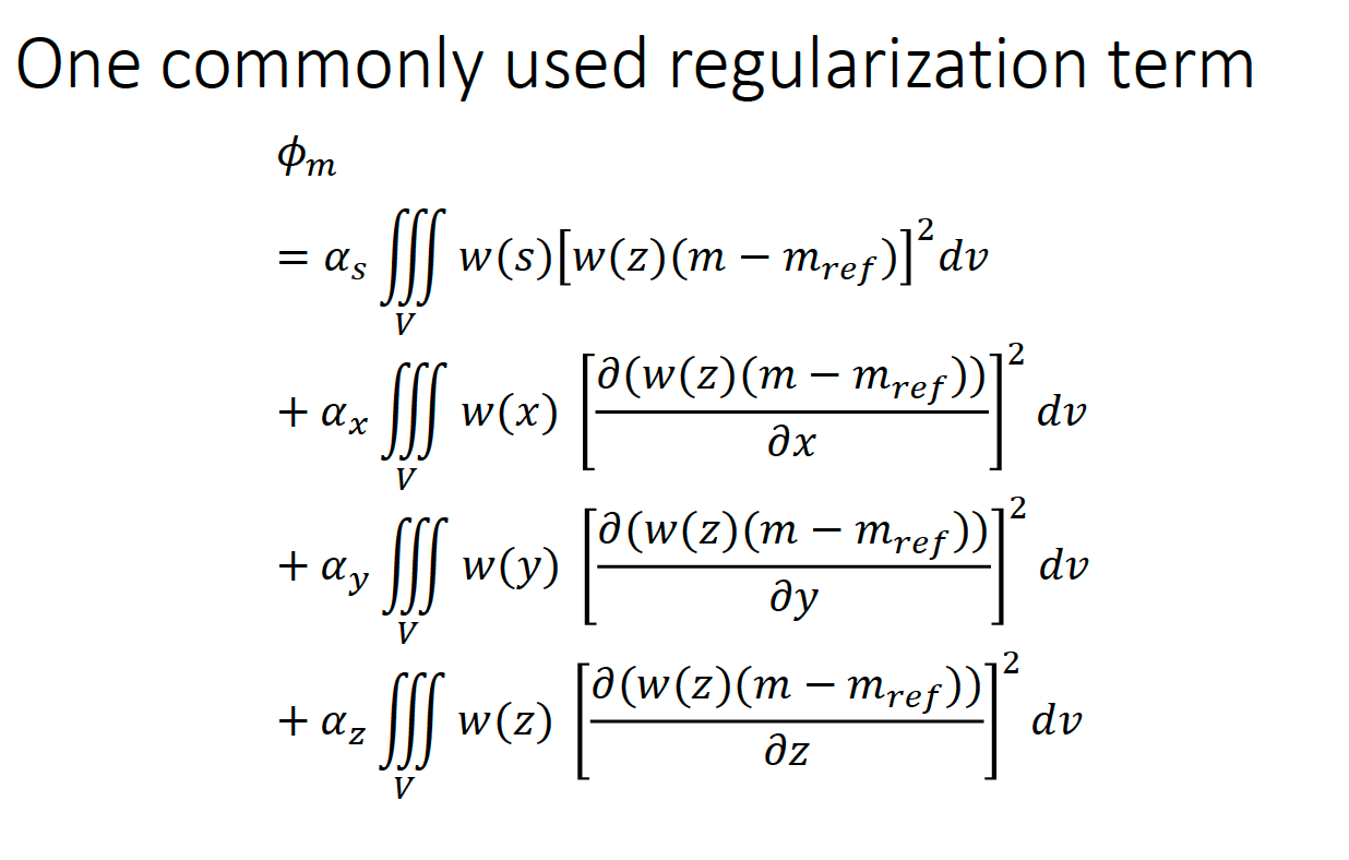
If we expand the model norm objective function into 3D model that means the flattest model norm will be calculated in x, y, z direction, respectively. The mathematical equation is expressed in the figure below:

One common used regularization term for 3D inversion.

7.2.3.2. Bound constraint

Bound constraint is another way to deal with non-uniqueness problem. As we mentioned before, inversion can be regarded as an optimization problem corresponding to minimize an objective function shown below:

$\phi(m)=\left\|d-Am\right\|_2^2+\lambda\left\|m\right\|_2^2$

Subject to $L\leq m\leq U$ .

The $L$ and $U$ are lower and upper bounds respectively. So the inverted physical property value will be constraint between $L$ and $U$ .

7.2.4. depth weighting

For example, let’s assume a dipping tilted body with a density of 1 g/cc. The gravity gradient data can be seen in the second column on the right of the following picture (in gzy, gzx, gzz). We then use those three data to do an inversion and recover the dipping body.

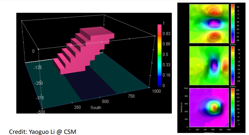
*(left) the true density model and (right) the gravity gradient data*

In a generic inversion scheme (inversion without bound constraint or depth weighting), the recovered density will behave similarly as the inverted model seen in the following image. Notice that the recovered density model is concentrated at the top of the surface. Furthermore, there are negative densities in the recovered density model, even though the true dipping model does not contain any negative values. This is because the gravity gradient data that we use (gzy, gzx, gzz) contains negative values, thus introducing negative values in the recovered/inverted density model. The dipping shape of the true model is not recovered in the inverted result as well.

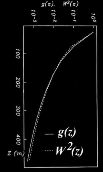
*(left) recovered model from inversion (right) true model*

The reason why the density values are concentrated on the surface is because of the behavior of the kernel function. The kernel function for potential fields (be it magnetic or gravity) always decreases with depth. The inverse solution is a combination of the kernels, and therefore, this behavior affects the inversion result as well (i.e. the recovered density values decreases with depth). To counteract this, we can design a depth weighting function that decays with depth, similar to how the kernel function decays. We can design a weighting function W(z) that consistent with how g(z) is decaying (captures the decay of the kernels). This strategy is called depth weighting. For example, the following can be used as depth weighting:

$w(z) = \frac{1}{(z+z_0)^3}$

Where $z_0$ is the least-squares fit between g(z) and $w^2(z)$ , and z is the depth of the center of the model cell. From the following graph, we can see how similar $w^2(z)$ behaves compared to g(z).

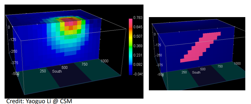
*plot of gravity (g(z)) and depth weighting (w(z)) [Li & Oldenburg 1996]*

When the depth weighting is applied correctly, the inverted model will be placed in the correct depth, as we can see in the following picture. Notice that the density values are not concentrated on the surface anymore and the depth is closer to the true model.

Inversion result after applying depth weighting [Yaoguo Li @ CSM]

However, notice that the recovered model does not match the shape of the true model and expands towards the deeper depths. For this, we can use the bound constraints. For example, if we impose that the density should always be greater than zero and is constrained in a narrow density interval, then the following can be recovered:

*Recovered data after bound constraints is applied [Yaoguo Li @ CSM]*

We see that the dip, depth, and length of the true model is recovered in the inverted model. Thus, using both depth weighting and bound constraints is an important step in inversion for potential field data.

7.2.5. examples

In the following sections, we will be going over different examples for gravity and magnetic inversion.

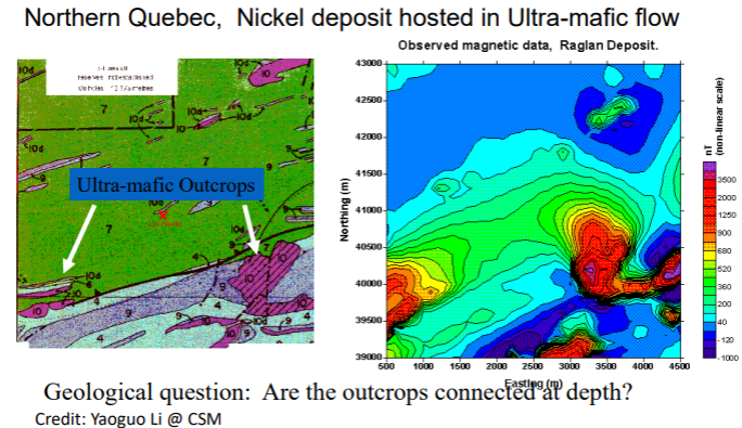
7.2.5.1. Raglan Deposit

The following image shows the contours of magnetic measurements of the Raglan deposit. The black outline indicates peridotite bodies. They are ultra-mafic and intrusive, and are known host for nickel deposit. Some of these ore bodies are associated with magnetic anomalies. The study area is focused on the bounded box in the image.

Contours of magnetic measurements in Raglan deposit

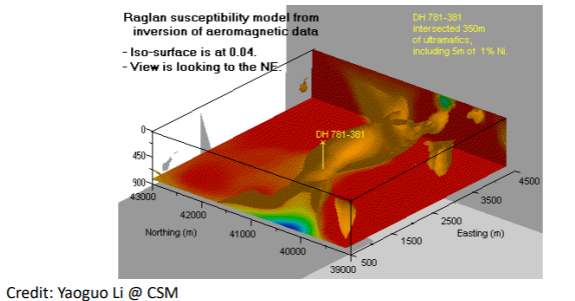
From the data, we can see a closure of the contours (i.e. magnetic highs) that corresponds to the ore bodies on the surface on the West, East, and South side of the box. The question is: are these bodies connected at depth? This question was solved using 3D inversion. After the 3D inversion result in the following image, we see that the turns out, the bodies are connected. The 3D density distribution is indicated by the gold-colored body that are well-connected at depth.

*(left) geological map of the raglan deposit and (right) its magnetic data*

*3D inversion result of the raglan deposit*

7.2.5.2. Iron Exploration

The above image shows 3D gravity gradient inversion of iron deposit. It applied depth waiting and bound constraint, and the result is the recovered bodies of a quasi-geology model, where the different colors indicates different geology units.

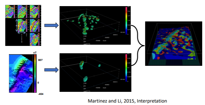
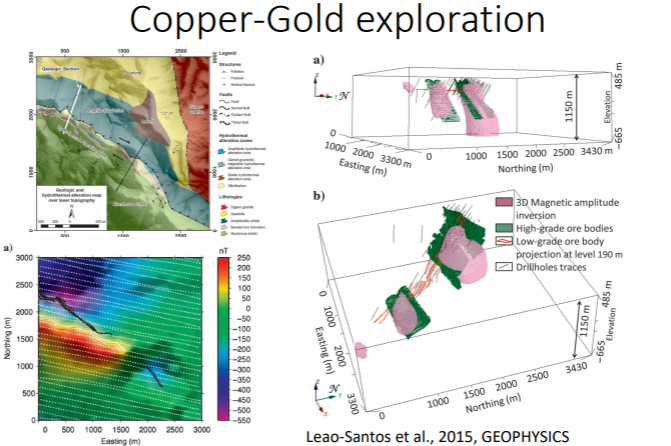
7.2.5.3. Copper-Gold Exploration

The following image is from airborne magnetic data. A 3D magnetic inversion is applied with depth weighting. From the image, the green color indicates data obtained from drill holes and the pink part is obtained from inversion.

*3D inversion of airborne magnetic data*

7.2.5.4. Diamond Exploration

Inversion succeeded in recovering the shape and depth of the kimberlite pipes (the smaller shapes that has vertical orientation in the following image)

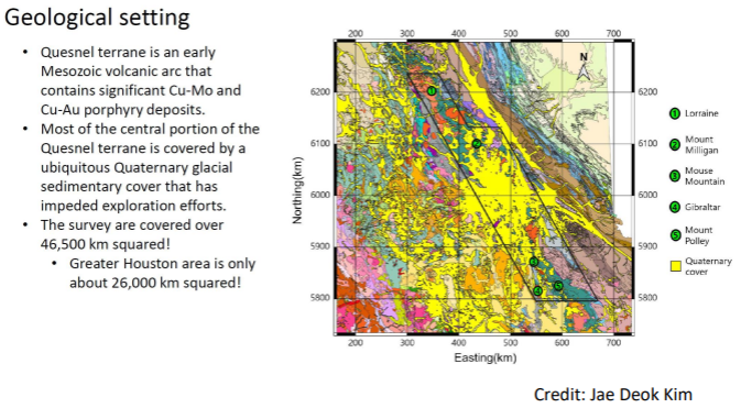
7.2.5.5. Regional Scale Exploration

From the following geologic map, the yellow parts are known as the quesnel terrain or the quartenary glacier. It is difficult to tell what geologic unit is underneath this terrain. In addition, the green part in the map refers to areas that are already producing copper-gold. With the close proximity of the quesnel terrain with the copper-gold deposits, it could be hypothesized that there could be copper-gold deposits underneath that terrain.

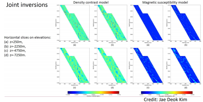
*Geologic map of a regional scale exploration area in Canada*

After using joint inversion (one type of inversion) of magnetic data and gravity data, the following image is obtained. Depth weighting is also applied in this case, however no bound constraints were applied because it is known that the susceptibility and density values can be negative in this area. After geology differentiation, it is found that the area around the Quesnel terrain might potentially be worth to look deeper into as potential copper-gold producer.

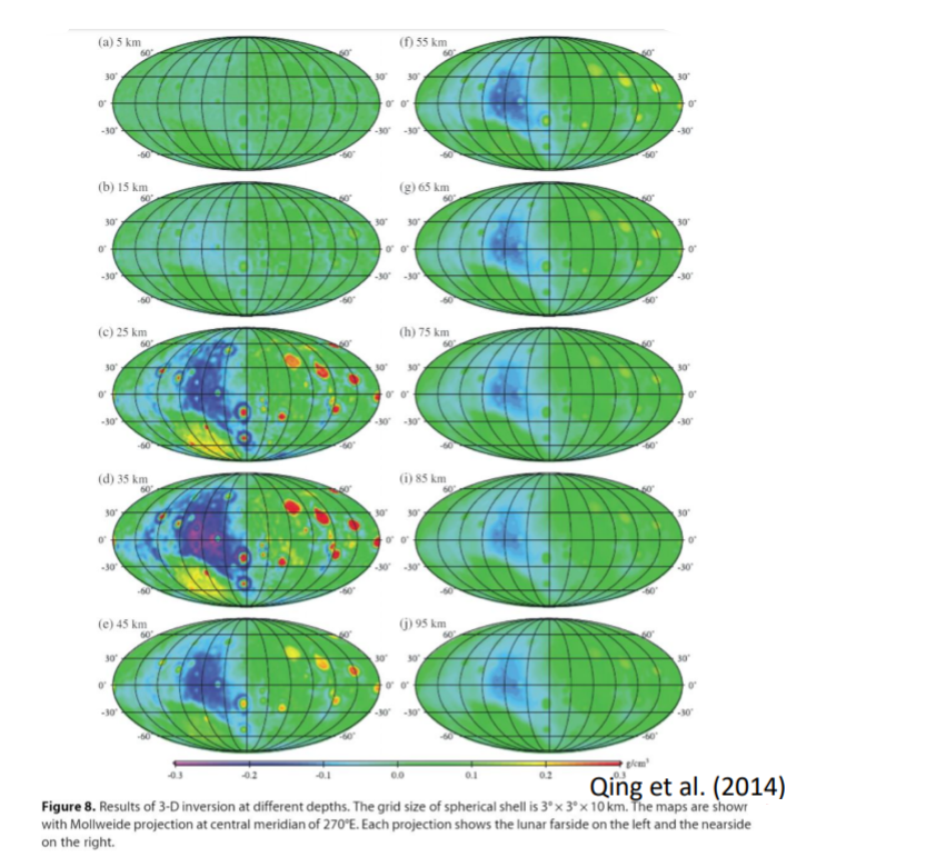
*Joint inversion result of the magnetic and gravity data in different depths*

7.2.5.6. The Moon

The 3D inversion of the moon used spherical coordinates because it covers for the whole planet (to accommodate the shape of the planet). The inversion core remains the same as the previously explained methods (i.e. depth weighting). From the following results, it can be seen that there are many mascon (mass concentrations) on the moon at certain depths.

*Inversion result of the moon [Qing et al., 2014]*

License

Icon for the Creative Commons Attribution-NonCommercial 4.0 International License