
9 Heat Engines. Refrigeration.
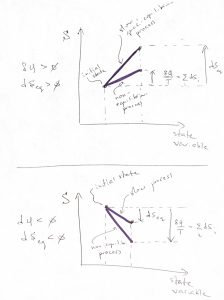
An important application of Thermodynamics and, arguably, the one that had motivated its systematic development in the first place, is Heat Engines. By construction, a heat engine consists of a working body, such as a gas or a mixture of vapor and liquid, that undergoes a cyclic process. During each cycle, heat that had been produced by some means is imparted to the working body. (The heat can be produced by burning a fuel, or a nuclear reaction, or by absorbing sunlight, etc.) Some of this heat is converted into useful work and some heat goes back in the environment. The temperature and entropy both vary during the cycle. We can graphically depict this state of affairs using the following graph:
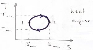
We have chosen the direction in the above process quite deliberately: The high-temperature,  leg of the process corresponds to inputting heat, while during the low temperature,
  leg, heat is extracted from the system. Under these circumstances, the net heat put into the system is positive:
(1) 
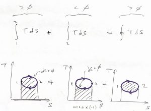
Indeed, the cyclic integral above can be presented as the sum of the integral along the leg and the leg:
(2) 
where we note that in the 1st integral in the r.h.s.,  , and in the 2nd integral,
  , because in the latter integral the argument decreases when going from the initial point of integration to the final point of integration. We next re-write the integrals so that the integration boundaries correspond with the numerical values of the argument at the left and right edge of the integration range, while being careful to specify the temperature along each leg:
(3) 
By construction,  . Likewise,
(4) 
(5) 
since for each value of entropy,  , by construction, and
  in the above integral. This notion can be illustrated graphically since the integral from left to right of a positive function is simply the area under the curve, while the integral of a positive function from right to left is equal to the area under the respective curve times the minus sign:
The fact of the total heat input being positive is key. To see this, integrate the differential form of energy conservation
(6) 
along the cycle:
(7) 
and note that the cyclic integral of the energy is equal to zero because, on the one hand, the integral of  yields
  for the process and, on the other hand, the energy is a state function. The value of a state function is fully determined by the values of the control variables irrespective of the preparation protocol of the system. Since the initial and final states for cyclic processes are identical,
  . Hence,
(8) 
and so we obtain that the work done by system is exactly equal to the total amount of heat absorbed by the working body:
(9) 
This equation can be regarded as a form of energy conservation law and implies that one cannot extract useful work out of nothing. Hypothetical engines that could do the latter, are called engines of the 1st kind. Clearly, such engines are physically impossible. Whenever there is an impression that work is created out of nothing, there a source of energy unaccounted for.
This simple and important result in 9 also presents an opportunity to explain why we have used the symbol  to denote small amounts of heat and work exchange, not the symbol “d”. This is to emphasize that heat and work are not state functions and how much heat or work has been exchanged with the systems actually depends on the specifics of the process, not just the initial and final states of the process. Here, specifically, we observe that neither
  nor
nor  individually corresponds to an increment of a function, but their difference,
  , does in fact correspond to an increment of a state function. One may also say that while one can ask how much energy a system has, one cannot ask how much heat (or work) the system has, only how much heat or work has been exchanged with the system during a specific process.
Eq. 9 is valid whether we go around the cycle clockwise or counterclockwise. In the former case, both integrals are positive, while in the latter, both integrals are negative. What type of machine does the counterclockwise process correspond to?
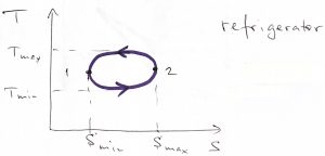
The negative work by the system means somebody else performs positive work on the system. At the same time, the negative  implies that the heat is imparted to the working body on the low temperature leg of the process and is extracted from the working body on the high temperature leg of the process. This state of affairs corresponds to refrigeration.
Thus the very same machine can be used both as an engine or a refrigerator depending on the directionality of the process. In practice, the engines work on much faster times scales than refrigerators and so one ordinarily employs distinct physical processes for the respective machines. Heat engines usually operate using hot gases. Although not particularly caloric in nature, expansion and compression of a gas can be done on rapid time scales thus allowing one to produce large amounts of power. For refrigerators, the power by itself is not of great priority. Instead, here one usually employs mechanical agitation or expansion to evaporate a liquid, which is in contact with the object or place that needs to be cooled. Evaporation extracts heat from that place. The vapor is then transported to elsewhere, where it condenses and gives off some of that heat. The liquid is then mechanically brought back in contact with the refrigerated object and so on. The power required to induce the evaporation is not particularly large, but the amount of heat involved in evaporation/condensation is substantial enough so that relatively small heat exchange units suffice to cool your home during hot Summer days.
Now, the efficiency of the heat engine is judged by which fraction of the heat imparted to the engine converted to useful work. Indeed, as far as the engine is concerned, the heat given off by the working body is not used to perform work by the engine itself. (This heat can be, in principle, collected and utilized.) Thus we define efficiency as
(10) 
which, by virtue of Eq. 9, becomes
(11) 
This can be expressed more vividly as the ratio of the following two areas:
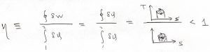
Because  , the efficiency is generally less than one but can be improved by lowering the temperature of the heat sink, i.e., the temperature at which the working body gives off heat, so at to make the quantity
  smaller in magnitude. It turns out that there is an intrinsic upper bound on the efficiency of a heat engine, as elucidated by the French engineer Sadi Carnot some 200 years ago. To establish this bound, we first state an upper bound on the heat that can be passed on to the system at temperature
  during an elemental process, known as the Clausius inequality:
(12) 
where is  is the eventual, equilibrium entropy change resulting from the process. The equality refers to the case when the system was, in fact, in equilibrium with the environment throughout the process, while the inequality covers situations where the process is faster than the relaxation time of the system.
The Clausius inequality comes about in the following way: Imagine the body has just received some heat in a process that is not necessarily quasi-static, in which case the body is not fully equilibrated. We can mentally subdivide the body into smaller parts, each of which still contains many molecules, but are small enough that it can be regarded as equilibrated. Thus the total amount of heat passed on to the system can be broken up into components  , for each of which we can use the equilibrium expression
  , and so:
(13) 
Suppose  and, thus, so are
  . In this case, the sum of the increments is maximized when the final value of
  is maximized. But is the total entropy the body, which achieves its maximum value in equilibrium:
(14) 
The  case can be treated similarly and gives the same result, as we graphically illustrate below:
Upon dividing 12 by and integrating along a cyclic process, one obtains the integral form of the Clausius inequality:
(15) 
because the equilibrium value of entropy is a state function and so  .
.
We can use Eq. 15 to place certain bounds on the heat exchange with the system along the high temperature and low temperature legs of the cyclic process:
(16) 
since  . Likewise,
(17) 
since is negative on this leg of the process and  . Adding these two inequalities yields:
(18) 
Where we used the Clausius inequality in the last step. In turn, this implies
(19) 
and, finally,
(20) 
or,
(21) 
To summarize, the quantity on the r.h.s. represents a fundamental upper bound on the efficiency of a (one-stage) heat engine. Note other sources of loss are present, such as friction between moving parts or incomplete burning of the fuel. This fundamental upper bound is intrinsically less than one, since the absolute zero of temperature,  , is not achievable. A hypothetical engine that would convert all of the heat into useful work is called the heat engine of the 2nd kind. Carnot’s result, then, demonstrates that the engine (or “perpetual motion”) of the 2nd kind is impossible. This notion is yet another equivalent formulation of the 2nd Law of Thermodynamics.
The natural question is, then: Aside from those additional losses, is there a process where the maximum possible value of  , i.e.
  , is in fact achieved? Upon inspection of Eqs. 16 and 17 we readily conclude that the equality in those two equations are achieved when
  throughout the high temperature leg, and
  throughout the low temperature leg. This is achieved only in the following cycle, which is called the “Carnot cycle”:
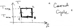
That is, the temperature should actually stay constant during heating exchange. It is instructive to re-plot this cycle in the pressure-volume plane, to see where the working body expands and where it contracts. In the  plane, the cycle looks more complicated because the straight lines connecting the corners of the rectangle in the
  plane become curved lines in the plane. Indeed, the isotherm becomes
  , the isotherm becomes
  . The isentropes
  and
and  becomes curves along each of which the quantity
  remains constant. This is made apparent by setting
  in the expression for the entropy we had obtained earlier:
(22) 
and using the ideal gas law  .
.
One can convince oneself that if an isentrope and isotherm intersect at some point  , the isentrope always have a steeper slope than the isotherm, because
  . Thus we arrive at the following picture for the Carnot cycle in the plane:
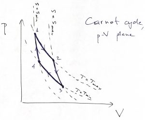
Thus we directly see that the system does useful work on the leg, where is expands isothermally and absorbs heat, and on the  leg, where it expands isentropically, i.e., without heat exchange with the environment, and, thus cools. On the
  leg, the system contracts and gives off heat while staying at the temperature of the heat sink, while in the final,
  leg, the system keeps contracting without heat exchange and, thus, warms back up to the temperature of the heat source.
Actual engines do not operate via the Carnot cycle for practical reasons, for which reason they are less efficient than what is prescribed by Carnot’s upper bound. (This is in addition to a variety of aforementioned mechanical and chemical losses.) Examples of those other types of engines are given below for your reference:
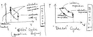
We note that since the electronic energies, which are of order eV, are much higher than the thermal energy scale, electrical engines operate much more efficiently than heat engines. Thus, in principle, if one can convert sunlight into electricity with relatively little heat dissipation, we can make convert energy into work in a drastically more efficient way. We know that absorption of light by molecules is accompanied by some vibrational relaxation, which leads to dissipation of energy. In any event, the best man-made photovoltaic devices can operate at 40% efficiency. Perhaps, plants can do it better.
Finally, we mention that these ideas can be applied to types of work other than mechanical work. Imagine, for instance, recurrent shuttling of ions across the membrane of a living cell or a mitochondrium:
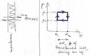
Here, one may consider a cyclic process where the temperature is kept constant, and so the appropriate thermodynamic potential is the Helmholtz free energy:  , (
, ( ). Hereby one can extract mechanical work
  , if the ions diffuse back and forth in a cyclic fashion while the two sides of the membrane are maintained at different values of the chemical potential. Conversely, one may induce ion transfer by mechanically moving the interface.
