The temperature. Heat Transfer. Equilibrium. Equipartition of energy. The Ideal Gas Law

Vassiliy Lubchenko

4 The temperature. Heat Transfer. Equilibrium. Equipartition of energy. The Ideal Gas Law

We begin this Chapter with a puzzler. Imagine the following setup, where a rigid, heat-insulated container is divided in two parts by a rigid piston that can freely move left of right. Each part contains a nearly ideal gas for which the following parameters are known: mass $m$ , concentration $n=N/V$ , and average velocity squared $\langle v^2 \rangle$ . The quantities pertaining to the l.h.s. are labeled with “1”, and to the r.h.s. with “2”.

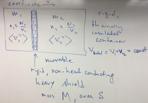
Clearly the ratio of the concentrations, $n_1/n_2$ is in one-to-one correspondence with the position of the piston and thus can be changed at will by moving the piston. Indeed, $n_1 = N_1/V_1$ , $n_2 = N_2/V_2 = N_2/(V_\text{total}-V_1)$ , where the total volume $V_\text{total}=V_1+V_2$ remains constant by construction. Thus, $n_1/n_2 =(N_1/N_2) (V_\text{total}-V_1)/V_1$ , where $(N_1/N_2)$ is fixed, also by construction.

Now the puzzler: Suppose we prepare the system so that the following conditions are satisfied:

(1) $\begin{equation*} n_1 m_1 \langle{v_1^2} \rangle \:=\: n_2 m_2 \langle{v_2^2} \rangle \end{equation*}$

while

(2) $\begin{equation*} m_1 \langle{v_1^2\rangle \: \neq \: m_2 \langle{v_2^2} \rangle \end{equation*}$

The puzzler is: Will the piston move or will it remain stationary? Is the system in true equilibrium or not?

We have seen in the preceding Chapter that the pressure

(3) $\begin{equation*} p \:=\: \frac{1}{3}\:m \langle{v^2}\rangle n \end{equation*}$

Suppose the area of the piston is $S$ . Thus, the net force acting on the piston:

(4) $\begin{equation*} f = p_1 S - p_2 S \:=\: (p_1 - p_2) S \end{equation*}$

should vanish by Eqns. (1) and (3). Thus the piston is in a state of mechanical equilibrium and should stay put. Or, should it?

Before we proceed further, a short comment regarding the term “nearly ideal gas”. In a nearly ideal gas, the particles are almost never in contact with one another and collide (interact) just often enough to “thermalize”, or randomize their motions so that the particles sample all possible values of the velocity and coordinate without any bias. As a result, any microscopic configuration will be visited again and again. This unbiased, recurrent sampling of a distribution that remains steady for an arbitrarily long time corresponds to a statistically steady, “equilibrated” system. In formal terms, equilibrium means that one may define a fixed, time-independent distribution for all the coordinates and velocities. Every quantity will fluctuate with in time, but the fluctuations each will be around a steady value:

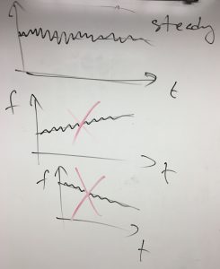
Only if this steady value remains steady forever, can we technically talk of “equilibrium”. In actuality, infinite observation times are unrealistic, and so when we say “infinite time”, we really mean “infinite, in principle”.

One useful property of a nearly ideal gas is that its energy is almost exclusively contained in the motion of the molecules, and almost none of it is stored in the potential energy:

(5) $\begin{equation*} E_\text{kin} \equiv \sum_i \frac{m_i v_i^2}{2} \gg V(\{\vec{r}_i\}) \end{equation*}$

where by $\{\vec{r}_i\}$ we denote the full set of the coordinates of the particles.

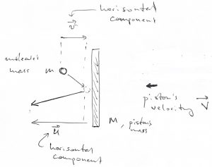
Now back to our puzzler. As in the preceding Chapter, we are interested only in the horizontal component of particle’s velocity. The shield can move exclusively horizontally, by construction. Let us again use a formula we derived in Chapter 2 to write down an expression for the velocity $u$ of particle that had just collided with a shield. The particle and the shield had velocities $v$ and $V$ , respectively, before the collision:

(6) $\begin{equation*} u\:=\:\frac{(m\:-\:M)v\:+\: 2MV}{m\:+\:M} \end{equation*}$

After we square this equation and average the resulting expression over the collisions—and, thus, over molecules—we obtain the following:

(7) $\begin{equation*} \langle{u^2}\rangle\:=\:\frac{(m\:-\: M)^2\langle{v^2}\rangle\:+\: 4M^2\langle{V^2}\rangle\:+\:4(m\:-\:M)\langle{vV}\rangle}{(m\:+\:M)^2}\end{equation*}$

Let us see now that in the approximation where the velocity of an incoming particle and the velocity of the shield just prior to the collision are uncorrelated, the average of the product $\langle{vV}\rangle$ breaks up into the product of the respective averages of the two factors:

(8) $\begin{equation*} \langle{vV}\rangle \: = \: \langle v \rangle \langle V \rangle \text{ if } v \text{ and } V \text{ are uncorrelated} \end{equation*}$

Digression on statistics: Uncorrelated variables. Suppose we have two distributed quantities, call them $x$ and $y$ . Completely analogously to how we handled a single variable case in the last Chapter, one can compute the average of any combination of two variables using a weighted average. For concreteness, consider the product $x \, y$ .

(9) $\begin{equation*} \langle x \, y \rangle \:=\: \sum_{k_1}^{M_1} \sum_{k_2}^{M_2} p_{k_1 k_2} \: x_{k_1} \: y_{k_2} \end{equation*}$

where we now sample two quantities, $x$ and $y$ . The quantity $p_{k_1 k_2}$ is the statistical weight (or proability) of a configuration where the variables $x$ and $y$ to simultaneously fall into a small rectangular sector $\Delta x_{k_1} \times \Delta y_{k_2}$ centered around the point $(x_{k_1}, y_{k_2})$ .

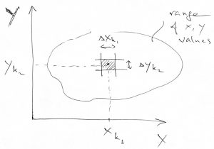
Because the variables $x$ and $y$ define a 2D space, these small rectangular sectors form a grid in that 2D space. Thus it is practical to use two indices to label those sectors. Other than this, the meaning of the weight $p_{k_1 k_2}$ is exactly the same as that of the weight $p_k$ we defined for a single distributed quantity in the last Chapter.

Next, let us see that the probabilities of uncorrelated events multiply:

(10) $\begin{equation*} p_{k_1 k_2} \:=\: p_{k_1}^{(1)} \: p_{k_2}^{(2)} \end{equation*}$

where the weight $p_{k_1}$ is the probability of outcome $x_{k_1}$ in a standalone experiment involving the variable $x$ and the weight $p_{k_2}$ is the probability of outcome $y_{k_2}$ in a standalone experiment involving variable $y$ . The superscripts $(1)$ and $(2)$ are simply labels we need to distinguish the distribution functions for the two variables, which are generally different. We begin a simple example of two fair coins, each of which, if tossed, will land heads up or tails up with equal probability 1/2. Clearly there are four equally likely outcomes for an experiment where the two coins are tossed at the same time:

coin 1

coin 2

heads

tails

heads

tails

Because there are 4 outcomes total and they are all equally likely, the probability of each outcome is exactly 1/4. For instance, the probability to get two tails at the same time is 1/4. On the other hand, the probability of getting tails for an individual fair coin is 1/2. Consistent with Eq. (10), $\frac{1}{2} \times \frac{1}{2} = \frac{1}{4}$ . By the same token, the probability to guess a 4-digit ATM code in one try is $\frac{1}{10,000}$ because there are 10,000 equally likely possibilities, i.e., numbers ranging from 0 to 9,999. Alternatively, one can look at this problem as the probability of guessing four uncorrelated one-digit numbers at the same time, again yielding $\frac{1}{10} \times \frac{1}{10} \times \frac{1}{10} \times \frac{1}{10} = \frac{1}{10,000}$ .

These ideas are not difficult to generalize to arbitrary, “unfair” coins. Suppose you are tossing an unfair coin, call it “coin 1”, which yields heads with probability $p^{(1)}_1 = 0.40$ (40%) and tails with probability $p^{(1)}_2 = 0.60$ (60%). Suppose also that your friend is tossing, entirely independently of you, a different unfair coin, call it “coin 2”, whose outcomes are heads with probability $p^{(2)}_1 = 0.70$ and tails with probability $p^{(2)}_2 = 0.30$ . Suppose you have tossed your coin a $N^{(1)}= 1000$ times. Let’s say your experiment yielded $N_1^{(1)} = 400$ heads. For each one of those heads, you know your friend had heads with probability $p^{(2)}_1 = 0.70$ , and so the number of outcomes that will count toward the “heads (coin 1) + heads (coin 2)” outcome, the top outcome entry in the Table above, is $N_1^{(1)} \times p^{(2)}_1 =400 \times 0.70 = 280$ . Thus the statistical weight of the “heads-heads” outcome is $\frac{N_1^{(1)} \times p^{(2)}_1}{N^{(1)}} = \frac{N_1^{(1)}}{N^{(1)}} \times p^{(2)}_1 = p^{(1)}_1 \times p^{(2)}_1 = 0.28$ . Likewise, the probability of the “tails (coin 1) + heads (coin 2)” outcome is $p^{(1)}_2 \times p^{(2)}_1 = 0.12$ and so on. We see that the multiplication of probabilities comes about because the success rate of a compound event is conditional on the success of both of the constituent events. When the constituent events are statistically independent, the success rates of the individual events must be simply multiplied in order for us to determine the overall success rate. For this very reason, by the way, the rate of bimolecular reaction is proportional to the product of the activities (or concentrations) of the individual reactants: One needs one of both species to create a product molecule.

The converse of the above logic is of equal significance for this class: If it turns out that the compound statistical weight of events 1 and 2 is not determined by simply multiplying their individual statistical weights, we may say that there is a statistical correlation, or, in more physical terms, “interaction” between the two degrees of freedom, such as $x$ and $y$ in an above example. In practice, we may not know beforehand whether there is any interaction. This, then, raises a question: How do we determine the individual statistical weights, in the first place? Here is how to do this. Assuming that we have performed enough experiments to sample all relevant configurations of the system, we can histogram the chances of a specific outcome for the degree of freedom 1 where the degree of freedom 2 was not even monitored but, hopefully, has adequately sampled all of its configurations. The resulting histogram is, then, simply the sum of the combined statistical weight over all configurations of the degree of freedom 2:

(11) $\begin{equation*} p_{k_1}^{(1)} = \sum_{k_2} p_{k_1 k_2} \end{equation*}$

Likewise,

(12) $\begin{equation*} p_{k_2}^{(2)} = \sum_{k_1} p_{k_1 k_2} \end{equation*}$

Note that, by construction, $\sum_{k_1} p_{k_1}^{(1)} = 1$ and $\sum_{k_2} p_{k_2}^{(2)} = 1$ , since each variable is guaranteed to assume some value with probability 1 (or, equivalently, 100%). This automatically ensures that the combined distribution $p_{k_1 k_2}$ is normalized, too:

(13) $\begin{equation*} \sum_{k_1} \sum_{k_2} p_{k_1 k_2} = 1 \end{equation*}$

This is particularly obvious when the two variables are statistically independent:

(14) $\begin{equation*} \sum_{k_1} \sum_{k_2} p_{k_1}^{(1)} \: p_{k_2}^{(2)} \:=\: \sum_{k_1} p_{k_1}^{(1)} \sum_{k_2} p_{k_2}^{(2)} \:=\: \sum_{k_1} p_{k_1}^{(1)} \times 1 = \sum_{k_1} p_{k_1}^{(1)} = 1 \end{equation*}$

The above equations illustrate, among other things, how to manipulate double sums where the summed object is factorizable into a product, where one factor depends exclusively on one summation variable and the other factor depends exclusively on the other summation variable. By the same token, we can now compute the average of the product of two independent variables:

(15) $\begin{eqnarray*} \langle x \, y \rangle \:&\equiv&\: \sum_{k_1}^{M_1} \sum_{k_2}^{M_2} p_{k_1 k_2} \: x_{k_1} \: y_{k_2} \:=\: \sum_{k_1}^{M_1} \sum_{k_2}^{M_2} p_{k_1}^{(1)} \: p_{k_2}^{(2)} \: x_{k_1} \: y_{k_2} \\ \:&=&\: \sum_{k_1}^{M_1} p_{k_1}^{(1)} x_{k_1} \sum_{k_2}^{M_2} p_{k_2}^{(2)} y_{k_2} \:=\: \sum_{k_1}^{M_1} p_{k_1}^{(1)} x_{k_1} \langle y \rangle \:=\: \langle y \rangle \sum_{k_1}^{M_1} p_{k_1}^{(1)} x_{k_1} \\ \:&=& \: \langle y \rangle \langle x \rangle \:=\: \langle x \rangle \langle y \rangle \end{eqnarray*}$

If you do not feel comfortable with this type of algebraic manipulations, it may be worthwhile to practice by writing out such double sums explicitly for small values of $M_1$ and $M_2$ .

Now, we can show, using the same logic as above, that the compound probability of three or more uncorrelated events also multiply. Indeed, one can relabel the compound experiment concerning, say, coin 2 and coin 3 as experiment 2 and repeat the argument. To summarize, for an arbitrary number of distributed variables, $N$ :

(16) $\begin{align*} p_{k_1 k_2 \ldots k_N} \:&=\: p_{k_1}^{(1)} \: p_{k_2}^{(2)} \times \ldots \times p_{k_N}^{(N)} \text{ variables uncorrelated, statistically independent} \\ p_{k_1 k_2 \ldots k_N} \:&\ne \: p_{k_1}^{(1)} \: p_{k_2}^{(2)} \times \ldots \times p_{k_N}^{(N)} \text{ variables correlated, interactions present} \end{align*}$

End of statistics digression.

Now that we have established the (approximate) validity of Eq. (8), we are ready to formulate conditions for true equilibrium. Indeed, in true equilibrium, the piston is not moving, on average: $\langle V \rangle = 0$ , which implies, by Eq. (8), that

(17) $\begin{equation*} \langle v V \rangle = 0 \end{equation*}$

Furthermore, in equilibrium, all directions in space must be equivalent or, else, there would be a net flow of particles or other properties. For example, suppose for a moment that two opposite directions are not equivalent in that the particle flux in one direction is not equal to the particle flux in the opposite direction. In that case, there would be a non-vanishing net flow along this direction which would, then, result in a continuing piling up of particles in one place and a continuing “drain” of particles in another place. In addition, the concentration should be on average spatially uniform, too, so as to also prevent a net flow. Because the flux is the product of the concentration and velocity, respectively, the velocities of individual particles should be distributed in a way that is independent of the place and direction. For this reason, we must conclude that the characteristics of the incoming and outgoing particles, near the “collision zone”, should be on average the same:

(18) $\begin{equation*} \langle u^2 \rangle = \langle v^2 \rangle \end{equation*}$

Eqs. (7), (17), and (18) then yield, after a bit of algebra, a remarkably consequential result:

(19) $\begin{equation*} \frac{m \langle v_x^2 \rangle}{2} = \frac{M \langle V_x^2 \rangle}{2} \end{equation*}$

where I have added the 1/2 factors for future convenience and the subscript $x$ to emphasize that we are dealing with motion along the coordinate axis $x$ . What Eq. (19) tells us that the kinetic energy of the motion of each particle and the piston must be mutually equal in equilibrium, on the average! Since this applies to the molecules on both sides of the piston, we conclude that in equilibrium,

(20) $\begin{equation*} \frac{m_1 \langle v_{x, 1}^2 \rangle}{2} = \frac{m_2 \langle v_{x, 2}^2 \rangle}{2} \end{equation*}$

Let us refocus on an individual compartment of our original setup. Since the directions $x$ , $y$ , and $z$ are all equivalent in equilibrium, one has it that

(21) $\begin{equation*} \frac{m\langle v_x^2 \rangle}{2}\:=\:\frac{m \langle v_y ^2 \rangle}{2}\:=\:\frac{m \langle v_z^2 \rangle}{2} \end{equation*}$

At the same time, the velocity vector can be decomposed into three mutually orthogonal components: $\vec{v}\:=\:v_x\vec{e_x}\:+\:v_y\vec{e_y}\:+\:v_z\vec{e_z}$

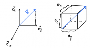
Thus

(22) $\begin{equation*} {v^2} \:=\: v_x^2 \:+\: v_y^2 \:+\: v_z^2 \end{equation*}$

By the way, because of this geometrical relation, the kinetic energy of motion in spatial dimensions greater than 1 is simply the sum of the kinetic energies of motion along individual directions:

(23) $\begin{equation*} \frac{m \langle v ^2 \rangle}{2} \:=\: \frac{m\langle v_x^2 \rangle}{2}\:+\:\frac{m \langle v_y ^2 \rangle}{2}\:+\:\frac{m \langle v_z^2 \rangle}{2} \end{equation*}$

In any event, Eq. (22) yields

(24) $\begin{equation*} \langle{v^2}\rangle\:=\:\langle v_x^2 \rangle\:+\: \langle v_y ^2\rangle\:+\:\langle v_z ^2\rangle \end{equation*}$

Which, then, leads, by Eq. (21), to :

(25) $\begin{equation*} \frac{m\langle v_x^2 \rangle}{2}\:=\:\frac{m \langle v_y ^2 \rangle}{2}\:=\:\frac{m \langle v_z^2 \rangle}{2} \:=\:\ \frac{1}{3} \: \frac{m \langle v ^2 \rangle}{2} \end{equation*}$

In view of Eq. (20), this yields that in equilibrium, the average kinetic energy of a molecule on the l.h.s and a molecule on the r.h.s., respectively, must be the same:

(26) $\begin{equation*} \frac{m_1 \langle v_{1}^2 \rangle}{2} = \frac{m_2 \langle v_{2}^2 \rangle}{2} \end{equation*}$

On the basis of Eq. (20) or (26) we then find the answer to the puzzler: The piston will actually move because the assumption of the piston being stationary is inconsistent with the condition (2). What gives?? After all, the piston appears to be in mechanical equilibrium, by Eq. (1)! The answer is that condition (1) only ensures that the net mechanical force on the piston vanishes only on the average, but not necessarily at any given moment. This uncompensated force, which fluctuates around zero, then leads to fluctuations in the position of the piston and a gradual drift either leftward or rightward, the direction depending on the sign of inequality in Eq. (2), to be determined shortly. Suppose, for concreteness, that in the beginning:

(27) $\begin{equation*} \frac{m_1 \langle v_{1}^2 \rangle}{2} \: > \: \frac{m_2 \langle v_{2}^2 \rangle}{2} \hspace{20mm} t=0 \end{equation*}$

To actually reach equilibrium, the piston should be moving in the direction such that the quantity $\frac{m_1 \langle v_{1}^2 \rangle}{2}$ should be decreasing over time, while the quantity $\frac{m_2 \langle v_{2}^2 \rangle}{2}$ should be increasing over time so as to meet somewhere midway by the time equilibrium is reached:

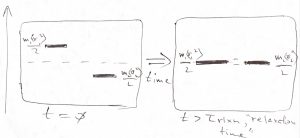
To understand what is happening physically, we note that the total kinetic energy of the gas on the l.h.s., $E_1 = N_1 \frac{m_1 \langle v_{1}^2 \rangle}{2}$ is decreasing, while the total kinetic energy of the gas on the r.h.s., $E_2 = N_2 \frac{m_2 \langle v_{2}^2 \rangle}{2}$ is increasing as the system is approaching equilibrium. In other words, the energy stored in the motions of the particles is being transferred, while no other property is being transferred at the same time. Indeed, the pressures in the two compartments are mutually equal (no momentum transfer) and there is no particle transfer either (the piston is impermeable by construction).

What do we make out of this type of energy transfer, where just the kinetic energy of the molecules’ motion is moved from one place to another, while no macroscopically observable quantity is transferred and there are no visible changes in the shape or position of the objects involved? This is the familiar heat transfer! The above argument also provides a simple criterion for the direction of heat transfer, if any: Heat will flow from places where the quantity $\langle m v^2/2 \rangle$ is greater to places where the quantity $\langle m v^2/2 \rangle$ is lower. This means the quantity $\langle m v^2/2 \rangle$ is a good proxy for what we call the temperature. In fact, by convention, we define temperature $T$ so that:

(28) $\begin{equation*} k_B T \:\equiv\: \frac{1}{3} \: \langle m v^2 \rangle \end{equation*}$

We have included the mass of the molecule inside the average to account for the possibility that more than one species can be present in the system. Recall that Eq. (26) was written with two pure gases separated by a partition, but applies equally well to a mixture of two nearly ideal gases. In any event, the above definition of the temperature is clearly not unique. Any other definition where $T$ is a monotonically increasing function of $\langle m v^2 \rangle/2$ would be workable, but the linear dependence in the above definition happens to be quite convenient, as we will have a chance to witness many times in the future.

The Boltzmann constant $k_B=1.38 \cdot 10^{-23}$ J/K, is just that: a numerical constant used to convert from temperature to energy. Really, temperature has the meaning of energy, consistent with its definition of being equal, up to a multiplicative constant, to the kinetic energy of molecules.

The numerical factor of $1/3$ in Eq. (28) is quite arbitrary as well, but it is the convention that must be followed consistently. With this convention, we obtain that the average kinetic energy of motion per single degree of freedom is exactly $k_B T/2$ :

(29) $\begin{equation*} \frac{ \langle m v_x^2 \rangle}{2} \:=\: \frac{ \langle m v_y^2 \rangle}{2} \:=\: \frac{ \langle m v_z^2 \rangle}{2} \:=\: \frac{1}{3} \: \frac{ \langle{m v^2}\rangle}{2} \:=\: \frac{k_BT }{2} \end{equation*}$

a fact often referred to as the the Equipartition Theorem. A “degree of freedom” is something whose configuration can be described by a single number. For, instance, motion in 3D space corresponds with three degrees of freedom. We can extend these notions to motions other than purely translational motions. For instance, a rotation around a fixed axis corresponds with a single degree of freedom. Indeed, one can think of such a rotation as a translation of a bead confined to moving in a circle:

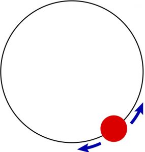
And so, for each rotation, there is a $k_B T/2$ worth of energy. Another classic example is a harmonic oscillator. This system has also a potential energy. We have seen, however, that on the average, the kinetic and potential energy of the harmonic oscillator are equal. Thus the total energy of a harmonic oscillator, on average is just the $k_B T$ . Non-withstanding the fact that these statements must be somtimes corrected for quantum-mechanical effects (and will be in due time), it is an incredibly useful notion that the typical thermal energy of a single degree of freedom is typically around $k_B T$ .

Next we combine Eq. (28) with the earlier derived relation for pressure: $p\:=\:\frac{1}{3} n m \langle{v^2}\rangle$ to obtain the Ideal Gas Law:

(30) $\begin{equation*} p \:=\:n k_B T \end{equation*}$

Note all the quantities in the above equation are intensive, i.e., provide no information about the size of the system. The concentration $n$ can be easily rewritten in terms of extensive variables, which, by definition, scale linearly with the system size. Indeed, $n = N/V$ , which, then, yields

(31) $\begin{equation*} p\:=\:\frac{N}{V} k_B T \end{equation*}$

or

(32) $\begin{equation*} p \, V\:=\:Nk_BT \end{equation*}$

Alternative ways to write down the Ideal Gas Law is

(33) $\begin{equation*} p \, V\:=\:\frac{N}{N_A} N_A k_B T \end{equation*}$

$\Rightarrow\: p \, V\:=\:\nu\:RT$

where $\nu \equiv N/N_A$ is the number of moles and $R \equiv k_B \cdot N_A = 8.31$ J/(mol K) is the universal gas constant. Also common, but unphysical way to write the ideal gas law is in terms of the molar volume $V_m \equiv V/\nu$ :

$p V_m\:=\:RT$

The Ideal Gas Law is both a definition of the temperature and a physical law. How does this work? We can use, as our “thermometer”, a specific gaseous substance that we think behaves like a nearly ideal gas and then make predictions about other gases. For instance, the ideal gas law allows one to predict the temperature of a gas, if its concentration and pressure are known. One, then, can compare this prediction by bringing test “test gas” in mechanical and thermal contact with our “thermometer gas” prepared at the same pressure and see, whether heat exchange will take place. In practice, we use thermometers that work using other physical phenomena. Nearly ideal gases are used to calibrate those more practical thermometers in a temperature range where we expect a gas behave nearly ideally. Making sure that temperature measurements are properly standardized in a broad temperature range requires much sophistication, engineering skill, and knowledge of Thermodynamics and Statistical and Quantum Mechanics.

We finish by returning to our puzzler. Suppose that the system was prepared so that $\frac{m_1 \langle v_{1}^2 \rangle}{2} \: > \: \frac{m_2 \langle v_{2}^2 \rangle}{2}$ , which we now know corresponds with $T_1 > T_2$ . Recall that the pressures remain fixed and mutually equal all along, as the mechanical equilibrium is never compromised: $p_1=p_2=\text{const}$ . Now, as the full equilibrium is approached and the two temperatures converge onto some value midway, the concentration of gas 1 must increase while the concentration of gas 2 must decrease with time, by the ideal gas law: $p_1=p_2 \Rightarrow \frac{n_1}{n_2} = \frac{T_2}{T_1}$ . This means that the piston will be moving to the left until equilibrium is achieved. One can further use energy conservation to connect the temperatures of the two gases to the eventual temperature $T_\text{f}$ of the system, i.e., after the piston attains its equilibrium position. Indeed, $\frac{3}{2}(N_1 k_B T_1 + N_2 k_B T_2) =\frac{3}{2}(N_1 + N_2) k_B T_\text{f}$ . The quantity $T_\text{f}$ is, of course, fixed. Combining this with the requirement that the pressures on the opposite sides of the piston are mutually equal, $N_1 T_1/V_1 = N_2 T_2/V_2$ , and that the total volume $V_1+V_2=V$ stays constant, we obtain that $\frac{N_1 T_1}{V_1}=\frac{(N_1+N_2) T_\text{f}-N_1 T_1}{V-V_1}$ . Simplifying this yields $\frac{N_1 T_1}{V_1}=\frac{N T_\text{f}}{V}$ , where $N\equiv N_1+N_2$ is the total particle number, a fixed quantity, of course. Consequently, we obtain that the pressure in the l.h.s. section $p_1=\frac{N_1 T_1}{V_1}$ will stay constant as the piston is drifting toward its eventual, equilibrium position. And so will the pressure one the other side, since $p_2=p_1$ .

Final remark: We assumed above that the piston is truly rigid to drive home the point that if one neglected thermal fluctuations, one would miss a very important aspect of equilibration in the form of heat exchange. In reality, a piston would have to be made out of molecules, too, and so it would conduct heat much more efficiently than the idealized piston we had in mind. Depending on how well the piston conducts heat, the temperatures in the respective compartments may not be actually uniform. These minor complications are not show stoppers and would distract us from the meat of the argument. Also, we did not mention that the piston’s coordinate and velocity would be fluctuating not just in one, but in all spatial directions, again because of the equipartition.

Advanced Reading:

The total kinetic energy of a collection of particles can be presented as a sum of the kinetic energy of the center of mass, the pertinent mass given by the total mass of the system, and the total kinetic energy of the motion of individual particles relative to the center of mass. Indeed, we recall that the center-of-mass velocity is defined as $v_\text{CM} \equiv \frac{\sum_i m_i v_i}{\sum_i m_i}$ , where the sum $\sum_i m_i$ is simply the total mass of the system, of course. We rewrite this as $(\sum_i m_i) v_\text{CM} = \sum_i m_i v_i$ . Now consider the following expression, where we add together the kinetic energy of the center of mass, while setting the mass at the total mass of the system, and the kinetic energies of the individual particles in the reference frame attached to the center of mass:

(34) $\begin{equation*} \frac{1}{2} \left(\sum_i m_i \right) v^2_\text{CM} + \sum_i \frac{1}{2} m_i \left(v_i-v_\text{CM} \right)^2 = \left( \sum_i \frac{1}{2} m_i v_i^2 \right) + v_\text{CM} \left[ (\sum_i m_i) v_\text{CM} - \sum_i m_i v_i \right] \hspace{5mm} \end{equation*}$

Since the expression in the square brackets vanishes, as we just saw, one obtains:

(35) $\begin{equation*} \frac{1}{2} \left(\sum_i m_i \right) v^2_\text{CM} + \sum_i \frac{1}{2} m_i \left(v_i-v_\text{CM} \right)^2 = \sum_i \frac{1}{2} m_i v_i^2 \end{equation*}$

Per equipartition theorem, should the first term on the l.h.s. should be worth $3k_B T/2$ on the average?

License

Icon for the Creative Commons Attribution-NonCommercial-NoDerivatives 4.0 International License

Basic Notions of Thermodynamics and Quantum Mechanics for Natural Sciences Copyright © 2020 by Vassiliy Lubchenko is licensed under a Creative Commons Attribution-NonCommercial-NoDerivatives 4.0 International License, except where otherwise noted.

License

Share This Book