Gibbs Free Energy, Entropy of Mixing, Enthalpy, Chemical Potential, Gibbs-Duhem

Vassiliy Lubchenko

8 Gibbs Free Energy, Entropy of Mixing, Enthalpy, Chemical Potential, Gibbs-Duhem

Next we determine the thermodynamic potential that controls the equilibration of the volume, in addition to controlling the equilibrium value of the energy. In many, of not most cases of interest, the volume of the system cannot be rigidly controlled. Instead, we can only be sure of the value of the pressure. For instance, most liquids do not fill their container fully, and so even if the container is completely rigid (which is an idealization) and fully sealed, the liquid will occupy only a portion of the container, the rest occupied by its vapor or the corresponding crystal. In an open container, clearly one can only control the pressure.

Perhaps the easiest way to determine the pertinent thermodynamic potential is to first write down the energy conservation law in a form that brings out the energy and volume dependence of the entropy:

(1) $\begin{equation*} dS \:=\: \frac{1}{T} dE \:+\: \frac{p}{T} \, dV \end{equation*}$

We are mindful that the above equation pertains to the equilibrium values of all the quantities. Thus in equilibrium,

(2) $\begin{align*} \left(\frac{\partial S}{\partial E}\right)_{V,N} &= \frac{1}{T} \\ \left(\frac{\partial S}{\partial V}\right)_{E, N} &= \frac{p}{T} \end{align*}$

and, hence,

(3) $\begin{equation*} 1 - T \left(\frac{\partial S}{\partial E}\right)_{V,N} =0 \end{equation*}$

(4) $\begin{equation*} p - T \left(\frac{\partial S}{\partial V}\right)_{E, N} = 0 \end{equation*}$

Note we have explicitly indicated that the particle number $N$ is being kept constant, which will be of use later one.

Recall that Eq. 3 resulted from minimizing the function $\tilde{A} \equiv E - TS(E, V)$ with respect to $E$ . It is not hard to see that Eq. 3 results just as well from minimization with respect to $E$ of the following function

(5) $\begin{equation*} \tilde{G} \:\equiv \: E \,+ \, p \, V \,- T \, S(E, V, N) \end{equation*}$

At the same time, we can readily convince ourselves that minimizing this function with respect to $V$ also yields Eq. 4! To be clear, the parameters $T$ and $p$ are kept constant during the minimization as well. The function $\tilde{G}$ , then, represents the sought thermodynamic potential governing the fluctuations of both the energy and volume when the temperature and pressure are externally imposed. Just as for the thermodynamic potential $\tilde{A}$ , there are two ways to interpret Eq. 2: On the one hand, they tell us the values of temperature and pressure that are needed to achieve specific equilibrium values for the energy and volume. On the other hand, given specific values of externally imposed temperature and pressure, the equilibrium energy and volume correspond to the minimum of the function $\tilde{G}$ , where Eq. 2 expresses the formal condition for the location of the minimum on the $\tilde{G}$ surface. As an example, we show the $\tilde{G}$ surface for the ideal gas:

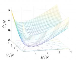
where we used the expression

(6) $\begin{equation*} S(E, V, N) - S^\ominus \:=\:N \, c_V \ln\left(\frac{E}{N c_V T^\ominus}\right) \:+\:N k_B \ln\left(\frac{V}{V^\ominus}\right) \end{equation*}$

obtained by taking the $S(V, T, N)$ dependence derived in the last Chapter:

(7) $\begin{equation*} S(T, V) - S(T^\ominus, V^\ominus) \:=\: C_V \ln\left(\frac{T}{T^\ominus}\right) \:+\:N k_B \ln\left(\frac{V}{V^\ominus}\right) \end{equation*}$

and substituting $C_V=N c_V$ and $T=E/C_V=E/(N c_V)$ . Note we must use the entropy as a function of energy, volume, and particle number $S=S(E, V, N)$ for both $\tilde{A}$ and $\tilde{G}$ ! In the graph, we set $T=1$ and $p=1$ and note that the precise choice of $S^\ominus$ , $T^\ominus$ , and $V^\ominus$ affects only the vertical, but not the lateral position of the graph. Thus, the positions of the minima are not affected. Lastly, it is convenient to graph extensive quantities per particle.

In the situation where $T$ and $p$ stand for externally imposed temperature and pressure and we are considering fluctuations of energy and volume, it is easy to see that such fluctuations will be subject to a restoring force if the curvature of the $\tilde{G}$ surface is positive throughout. We have already discussed the stability with respect to energy fluctuations in the preceding Chapter and postpone further discussion of the necessary criteria until the next Chapter.

Similarly to how we defined the Helmholtz free energy as the minimum of the $\tilde{A}$ potential, we now define the Gibbs free energy as the minimum of the $\tilde{G}$ function:

(8) $\begin{eqnarray*} G &\equiv& \tilde{G}(E_\text{mp}(T, p, N), V_\text{mp}(T, p, N), T, p, N) \\ & =& E_\text{mp}(T, p, N) - T S[E_\text{mp}(T,V), V_\text{mp}(T, p, N), N] + p\, V_\text{mp}(T, p, N) \end{eqnarray*}$

or, simply,

(9) $\begin{equation*} G \:\equiv \: E - T \, S + p \, V \end{equation*}$

where it is understood that every quantity is at its equilibrium value and, as such, is a function of exactly three independent quantities. A natural—but not unique!—choice of the variables is $T$ , $p$ , and $N$ .

We are now ready to formulate yet another version of the 2nd Law of Thermodynamics, i.e, that at constant pressure and temperature, a large system will spontaneously and irreversibly relax so as to minimize its Gibbs free energy. Once equilibrated, the system will remain in equilibrium indefinitely. This form of the 2nd Law is particularly useful because $T, p =\text{const}$ conditions are particularly common in experiment.To avoid confusion, we point out that although the equilibration of the system is all but inevitable, the 2nd Law, by itself, does not provide guidance as to the kinetics of the equilibration. These kinetics may, in fact, be rather slow. For instance, the stable form of solid carbon at normal conditions is graphite, not diamond. Yet diamond is incredibly stable, as we all know. Likewise, liquid glycerol can be stored on the shelf for decades, at normal conditions, yet its stable form at normal conditions is a crystalline solid!

As a simple yet useful illustration of the utility of the $p, T = \text{const}$ form of the 2nd Law, let us convince ourselves that gaseous mixtures essential never de-mix. Imagine two distinct, nearly ideal gases occupying two sides of a container separated by a movable, thermally conducting partition. The partition is also weakly permeable to both gases. Note these properties guarantee eventual equilibration: mechanical, thermal, and with respect to particle exchange. Suppose the gases occupy volumes $V_1$ and $V_2$ and are maintained at the same temperature and pressure.

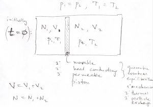
Thus, according to the ideal gas law, the particle numbers must be proportional to the respective volumes:

(10) $\begin{equation*} \frac{N_1}{N_2} = \frac{V_1}{V_2} \end{equation*}$

Thus the mole fractions of the two gases are, respectively

(11) $\begin{equation*} x_1 \:\equiv\: \frac{N_1}{N_1+ N_2} = \frac{V_1}{V_1 + V_2} \end{equation*}$

and

(12) $\begin{equation*} x_2 \:\equiv\: \frac{N_2}{N_1+ N_2} = \frac{V_2}{V_1 + V_2} \end{equation*}$

Note $x_1+x_2=1$ .

Clearly, both the thermal and mechanical equilibrium are in place, but the system is not in full equilibrium: Since the concentrations of each gas differ on the opposite sides of the partition, there will be uncompensated fluxes of both kinds of particles until the mixture will have the same composition in both parts of the container. No quantity in Eq. 9 will change as a result of the particle exchange except for one: the entropy. As a result of the mixing, the volume of gas 1 will increase from $V_1$ to $(V_1+V_2)$ and the volume of gas 2 will increase from $V_2$ to $V$ . The resulting entropy change is, then,

(13) $\begin{eqnarray*} \Delta S_\text{mix}/k_B &= &\left[ N_1 \ln\left(\frac{V_1+V_2}{V^\ominus}\right) \,+\, N_2 \ln\left(\frac{V_1+V_2}{V^\ominus}\right) \right] \\ &-& \left[ N_1 \ln\left(\frac{V_1}{V^\ominus}\right) \,+\, N_2 \ln\left(\frac{V_2}{V^\ominus}\right) \right] \\ &=& \left[ N_1 \ln\left(\frac{V_1+V_2}{V_1}\right) \,+\, N_2 \ln\left(\frac{V_1+V_2}{V_2}\right) \right] \\ &=& (N_1+N_2)\left[ \frac{N_1}{N_1+N_2} \ln\left(\frac{V_1+V_2}{V_1}\right) \,+\, \frac{N_2}{N_1+N_2} \ln\left(\frac{V_1+V_2}{V_2}\right) \right] \end{eqnarray*}$

In terms of the mole fraction $x$ and the total particle number $N \equiv N_1 + N_2$ , this expression looks particularly appealing:

(14) $\begin{equation*} \Delta S_\text{mix}/k_B \:=\: -N ( x_1 \ln x_1 \,+\, x_2 \ln x_2 ) \end{equation*}$

One can likewise derive that for an arbitrary mixture of ideal gases,

(15) $\begin{equation*} \Delta S_\text{mix}/k_B \:=\: -N \sum_i x_i \ln x_i \end{equation*}$

a celebrated formula, due to Gibbs.

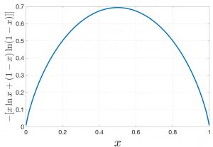
One can easily convince oneself that the mixing entropy is always positive, which we will do here graphically for the binary mixture from Eq. 14 while remembering that $x_2=1-x_1$ . The mixing entropy vanishes only for pure substances, $x_1=0$ or $x_2=0$ , of course and is maxed out at $k_B \ln 2$ per particle for an equal mixture $x_1=x_2=1/2$ :

The corresponding Gibbs free energy change is, then, always negative:

(16) $\begin{equation*} \Delta G_\text{mix} \:=\: - T \, S_\text{mix} < 0 \end{equation*}$

To appreciate just how unlikely de-mixing would be, we compare the probability of the mixed vs. de-mixed state. As in the preceding Chapter, the ratio of the numbers of accessible states is given by the exponential of the free energy times $(\-\beta)$ , the pertinent free energy being is that due to Gibbs, because we are keeping fixed temperature and pressure:

(17) $\begin{equation*} \frac{Z_\text{mix}}{Z_\text{de-mix}} \:=\: e^{-\beta \Delta G_\text{mix}} \:=\: e^{S_\text{mix}/k_B} \end{equation*}$

For one mole worth of a 50/50 mixture this would yield $\sim e^{4 \cdot 10^{23}}\sim 10^{10^{23}}$ , a grotesquely large number. To put this in perspective, I quote here the well known French mathematician Borel (by way of G.N.Lewis’s book “The anatomy of Science”): “Imagine a million monkeys allowed to play upon the keys of a million typewriters. What is the chance that this wanton activity should reproduce exactly all of the volumes which are contained in the library of the British Museum? It certainly is not a large chance, but it may be roughly calculated, and proves in fact to be considerably larger than the chance that a mixture of oxygen and nitrogen will separate into the two pure constitutents.”

Now, the aforementioned choice of the quantities $T$ , $p$ , and $N$ as the arguments of $G$ is natural not only in view of the definition of the Gibbs energy as the minimum of the $\tilde{G}$ function at fixed $p$ , $T$ , and $N$ , but also because of the fact that the partial derivative of $G$ w.r.t. these variables are particularly simple. To discuss this point in a more general way, let us revisit energy conservation while including the possibility that the particle number is allowed to change. For this, let us define a new quantity, called the chemical potential. The chemical potential is the energy cost of adding a particle to the system while no heat exchange takes place and no mechanical work is done: $\mu \:\equiv\: [ E(N+1) - E(N) ]_{S, V}$ . We note that $E(N+1) - E(N)=\frac{E(N+1) - E(N)}{1} = \frac{E(N+1) - E(N)}{(N+1)-N}$ . Under the assumption that the energy is a smooth function of the particle number $N$ , this ratio can be re-written as the following derivative:

(18) $\begin{equation*} \mu \:\equiv\: \left(\frac{\partial E}{\partial N}\right)_{S, V} \end{equation*}$

(There are certain issues with treating the intrinsically discrete variable $N$ as continuous, but they can be addressed systematically, see the Bonus and Advanced Discussions at the end of this Chapter.)

We can now write the energy conservation for systems with a variable particle number:

(19) $\begin{equation*} dE \:=\: T dS \:-\: p \, dV \:+\: \mu \, dN \end{equation*}$

or, equivalently,

(20) $\begin{align*} T &= \left(\frac{\partial E}{\partial S}\right)_{V, N} \\ -p &= \left(\frac{\partial E}{\partial V}\right)_{S, N} \\ \mu &= \left(\frac{\partial E}{\partial N}\right)_{S, V} \end{align*}$

Note that at this point, we are still considering pure systems, i.e., those containing just one chemical species. Mixtures will be considered in due time.

Thus for the increment of the Gibbs free energy we obtain

(21) $\begin{equation*} dG \:= \: d(E-TS+pV) \:=\: dE - d(TS) + d(pV) \: = \: dE - (TdS+SdT) + (pdV+Vdp) \end{equation*}$

which leads, in view of Eq. 19, to

(22) $\begin{equation*} dG \:=\: -SdT \:+\: V \, dp \:+\: \mu \, dN \end{equation*}$

or, equivalently,

(23) $\begin{align*} -S &= \left(\frac{\partial G}{\partial T}\right)_{p, N} \\ V &= \left(\frac{\partial G}{\partial p}\right)_{T, N} \\ \mu &= \left(\frac{\partial G}{\partial N}\right)_{T, p} \end{align*}$

Likewise, the increment of the Helmholtz energy, $A=E-TS$ , for a system with a variable particle number becomes

(24) $\begin{equation*} dA \:=\: -SdT \:-\: p \, dV \:+\: \mu \, dN \end{equation*}$

or, equivalently,

(25) $\begin{align*} -S &= \left(\frac{\partial A}{\partial T}\right)_{V, N} \\ -p &= \left(\frac{\partial A}{\partial V}\right)_{T, N} \\ \mu &= \left(\frac{\partial A}{\partial N}\right)_{T, V} \end{align*}$

And, finally we introduce a new function, called the enthalpy, or the heat function:

(26) $\begin{equation*} H \:=\: E \:+\: p\, V \end{equation*}$

Since $dH = d(E+pV) = dE + pdV + Vdp$ , one obtains

(27) $\begin{equation*} dH \:=\: TdS \:+\: V \, dp \:+\: \mu \, dN \end{equation*}$

or, equivalently,

(28) $\begin{align*} T &= \left(\frac{\partial H}{\partial S}\right)_{p, N} \\ V &= \left(\frac{\partial H}{\partial p}\right)_{S, N} \\ \mu &= \left(\frac{\partial H}{\partial N}\right)_{S, p} \end{align*}$

The increments of all four energy functions given above display a clear pattern: They all have simple-looking derivatives for certain choices of independent parameters, as summarized in the Table below:

$E=E(S, V, N)$

$dE \:=\: T dS \:-\: p \, dV \:+\: \mu \, dN$

$A=A(T, V, N)$

$dA \:=\: -SdT \:-\: p \, dV \:+\: \mu \, dN$

$G=G(T, p, N)$

$dG \:=\: -SdT \:+\: V \, dp \:+\: \mu \, dN$

$H=H(S, p, N)$

$dH \:=\: TdS \:+\: V \, dp \:+\: \mu \, dN$

Other choices of variables are possible so long as

The number of the variables is exactly three.
At least one of those three variables corresponds to an extensive quantity. This is needed because each one of the four energies is an extensive quantity itself and so at least one of the variables must contain information as to the size of the system.

The converse of the item 2 is worth elaborating on: If expressed per particle, each of the four energies no longer depends on $N$ and, thus, is a function of exactly two variables. Both of these remaining variables cannot contain information about the system size and, thus, must be intensive. Now let us take every item in the 1st column of the table above and re-write it per particle. In those cases where one or both of the arguments are extensive variables, we must replace them with their intensive counterparts per particle:

(29) $\begin{align*} \frac{E}{N} &= \epsilon \left(\frac{S}{N}, \frac{V}{N} \right) \\ \frac{A}{N} &= a \left(T, \frac{V}{N} \right) \\ \frac{G}{N} &= g \left(T, p \right) \\ \frac{H}{N} &= h \left( \frac{S}{N}, p \right) \end{align*}$

One immediately notices that of the four energies, the Gibbs energy has the simplest $N$ dependence:

(30) $\begin{equation*} G\:=\:N \, g(p, T) \end{equation*}$

and so

(31) $\begin{equation*} \left(\frac{\partial G}{\partial N}\right)_{T, p} \:=\: g(p, T) \end{equation*}$

comparing this result with the bottom equation from Eq. 23, one immediately obtains $\mu=g(p, T)$ . In view of Eq. 30 this lead to the remarkable result that the chemical potential is, in fact, the Gibbs free energy per particle!

(32) $\begin{equation*} G\:=\:N \, \mu \end{equation*}$

It is also clear from the above discussion that only two intensive variables are independent, while any other intensive property can be expressed as their function. A useful instance of such a functional relation can be obtained by noticing that $dG = d(N \mu) = N d \mu + \mu dN$ and subtracting $dG = N d \mu + \mu dN$ from Eq. 22. This yields what is known as the Gibbs-Duhem equation:

(33) $\begin{equation*} N \, d\mu \:=\: -SdT \:+\: V \, dp\end{equation*}$

It becomes particularly lucid when written our in terms of quantities per particle, which is accomplished by dividing it by the particle number:

(34) $\begin{equation*} d\mu \:=\: -s \, dT \:+\: v \, dp\end{equation*}$

where $s \equiv S/N$ is the specific entropy and $v \equiv V/N$ specific volume. Every quantity in the above equation is intensive. Thus we obtain $s = - (\partial \mu/\partial T)_p$ etc., as just advertised.

Why do we call enthalpy the “heat function”? Because it directly reflects the amount of exchanged heat during an isobaric process. (“Isobaric” means “at constant pressure”.) Indeed, per Eq. 27,

(35) $\begin{equation*} (dH)_{p, N} \:=\: T \, dS \end{equation*}$

If, in addition, the temperature is kept constant as well, one can easily integrate this to obtain

(36) $\begin{equation*} (\Delta H)_{p, T, N} \:=\: T \, (\Delta S)_{p, T, N} \end{equation*}$

(Clearly, the system must change its volume during such a process!)

Another consequence of Eq. 35 is a useful expression for the heat capacity at constant pressure:

(37) $\begin{equation*} C_p \:=\: T\left( \frac{\partial S}{\partial T} \right)_p \:=\: \left( \frac{\partial H}{\partial T} \right)_p \end{equation*}$

This indicates that the enthalpy is essentially the constant-pressure analog of the energy.

Finally, one may also write down simple relations between the thermodynamic functions, such as

(38) $\begin{equation*} G \:=\: A \:+\: p\, V \end{equation*}$

or

(39) $\begin{equation*}G \:=\: H \:-\: S \, T \end{equation*}$

As an illustration of the utility of these and earlier expressions, let us determine the expression for the chemical potential of a single-component ideal gas. First re-write Eq. 19 as

(40) $\begin{equation*} dS \:=\: \frac{1}{T} dE \:+\: \frac{p}{T} \, dV \:-\: \frac{\mu}{T} \, dN \end{equation*}$

and so

(41) $\begin{equation*} -\frac{\mu}{T} \:=\: \left( \frac{\partial S}{\partial N} \right)_{E, V} \end{equation*}$

To use this formula, we must express the entropy as a function of the three variables $E$ , $V$ , and $N$ exclusively. (This means that any other quantity that could be involved in the available expression must be expressed through those three variables.) Just such an expression is available in Eq. 6. Differentiating it w.r.t. $N$ , while keeping $E$ and $V$ fixed, yields:

(42) $\begin{eqnarray*} -\frac{\mu}{T} &=& c_V \left[ \ln \left( \frac{E}{N c_V T^\ominus} \right) - 1 \right] +k_B \ln \left( \frac{V}{V^\ominus} \right) \\ &=& k_B \ln \left[ \left( \frac{E}{e N c_V T^\ominus} \right)^{c_V/k_B} \left( \frac{V}{V^\ominus} \right) \right] \end{eqnarray*}$

Here we use that $\ln x - 1 = \ln(x/e)$ , where $e \equiv \text{exp}(1)$ , and $y \ln x = \ln (x^y)$ . Substituting $E = N c_V T$ , one obtains a compact expression:

(43) $\begin{equation*} \mu \:=\: - k_B T \ln \left[ \left( \frac{T}{e T^\ominus} \right)^{c_V/k_B} \left( \frac{V}{V^\ominus} \right) \right] \end{equation*}$

which, again, emphasizes the role of $k_B T$ as the basic thermal energy scale for a particle, but modified to account for specific conditions. The above expression can be re-written for other combinations of parameters, using the equation of state. It can be also used to write down expressions for the thermodynamic functions. And so, for instance, for a process conserving the particle number, one gets

(44) $\begin{equation*} G-G^\ominus \equiv \Delta G \:=\: N \, \Delta \mu \end{equation*}$

The corresponding Helmholtz free energy is, by virtue of Eq. 38:

(45) $\begin{equation*} \Delta A \:=\: \Delta G \:-\: \Delta (p\, V) \end{equation*}$

Bonus Discussion. Formulas up to Eq.(45) were derived having in mind processes that conserve particles. Some care is needed to use them for processes that do involve changes in $N$ . Processes that do not conserve particle numbers are central in Chemistry: Reactants and products inter-convert while the reaction itself exchanges particles with the environment via evaporation, condensation/solvation of airborne gasses, precipitation of poorly solvable species, etc. In contrast with changes in energy and volume, which can be made arbitrarily small, changes in the particle number $N$ are intrinsically discrete. Thus, while two states with different volumes, for instance, can be made arbitrarily similar, two states with different particle numbers may be similar, but are strictly distinct. Cases when a quantity is intrinsically discrete—or “quantized”—must dealt using Quantum Mechanics. Here, we can weasel our way of this apparent complication by using a reference state in Eqs. (7) that does not explicitly specify the particle number:

(46) $\begin{equation*} S(T, V) - S(T^\ominus, V^\ominus) \:=\: C_V \ln\left(\frac{T}{T^\ominus}\right) \:+\:N k_B \ln\left(\frac{V/N}{v^\ominus}\right) \end{equation*}$

where the quantity $v^\ominus \equiv V^\ominus/N$ is the specific volume of the reference state. It can be, of course, expressed through the reference temperature and pressure $v^\ominus = k_B T^\ominus/p^\ominus$ and I remind that we are working with the ideal gas. Let us evaluate the entropy change due to a change in the particle number, at constant volume and temperature:

(47) $\begin{equation*} S(T, V, N_2) - S(T, V, N_1) \:=\: k_B \ln\left(\frac{(V/N_2 v^\ominus)^{N_2}}{(V/N_1 v^\ominus)^{N_1}}\right) \end{equation*}$

To find out how this rather complicated expression comes about, the reader is invited to read the rest of the Chapter.

Advanced Discussion.

There would seem to be nothing special about processes that do not conserve the particle number. Perhaps the simplest example of such a process is a leaky container. Yet a lack of particle conservation, if any, has a fascinating statistical aspect: it allows one, in principle, to label particles that are otherwise identical. Indeed, imagine a leaky container that typically lets out one particle at a time. An escaped particle can thus be singled out and labeled by its location, because the latter location is outside the container. In contrast, we had built our description on the assumption that particles inside the container are strictly identical and exchange places faster than any relevant experimental time scale, thus preventing one from labeling the particles using their location. To “patch” this apparent limitation of assuming intrinsic indistinguishability of chemically identical particles when the particle number is not conserved, we first note that making a small hole in the container automatically breaks the translational symmetry of space: Those particles that are the closest to the hole are different from the rest because they are the likeliest to escape first; the corresponding region that is likeliest to contribute a particle has a volume comparable to that occupied by one particle, on the average. Consequently we must concede that the volume relevant for statistics of identical particles is not the total volume but, instead, the specific volume, i.e., the volume per particle. In other words, a particle can be labeled—and thus distinguished from the other particles—so long as it is contained within a region comparable to the specific volume. Conversely, if a volume contains more than one particle, the particles lose their identities. As an informal example, think of two identical twins in one room. So long as you know the two are confined to two separate parts of the room, you can label the twins by their locations. If, instead, the twins move about, such labeling is no longer possible. The above notions—which underlie the famous Maxwell demon paradox, among other things—can be addressed systematically in Quantum Mechanics, see the last Chapter of these Notes. Here, we will limit ourselves to the simplest argument which already suffices for nearly ideal gases. The Helmholtz free energy is computed according to $A=-k_B T \ln Z$ , where $Z$ is the partition function. Let us first consider an ideal gas made up of $N$ distinct particles. The total number of thermally available states for our compound system is simply the product of the numbers of states available to the subsystems: $Z = z_1 \times z_2 \times \ldots z_N$ . If the particles are, instead, indistinguishable, the latter expression overcounts the number of available states by the number of possible permutations of the particles since all configurations obtained using such permutations are physically equivalent. (This is assuming no two particles are in the same quantum state, something we do not have to worry about at low densities such that the gas behaves as nearly ideal. Informally speaking, one cannot permute two particles that occupy the same spot.) Since the number of permutations of $N$ objects is equal to $N!$ , a good approximation for the total number of thermally available states is given by

(48) $\begin{equation*} Z = \frac{1}{N!} \prod^N_i z_i = \frac{z^N}{N!} \end{equation*}$

where $z$ is the partition function—i.e. the number of thermally available states—for an individual particle, if standalone. The partition function for an individual monatomic molecule, according to quantum mechanics, is given by

(49) $\begin{equation*} z = \frac{V}{\Lambda_\text{dB}^3} \end{equation*}$

where the quantity

(50) $\begin{equation*} \Lambda_\text{dB} \equiv \left( \frac{2 \pi \hbar^2}{m k_B T} \right)^{1/2} \end{equation*}$

is the so called de Broglie wavelength. This quantity gives the localization length of a particle at thermal energy. In a sense, the partition function (49) provides the number of distinct spots a particle in equilibrium with its environment can occupy. Using the Stirling approximation, $\ln N! \approx N \ln N -N$ , which is valid for $N \gg 1$ , we obtain for a monatomic gas:

(51) $\begin{equation*} A = -k_B T \ln Z = -k_B T \ln \frac{z^N}{N!} \approx - N k_B T \ln \left( \frac{z e}{N} \right) = -N k_B T \ln \left( \frac{z e}{N} \right) \end{equation*}$

and so, finally, we obtain that the volume entering the expression for the Helmholtz free energy is the specific volume, not the total volume, as anticipated earlier:

(52) $\begin{equation*} A = - N k_B T \ln \left( \frac{V}{N} \frac{e}{\Lambda_\text{dB}^3} \right) \end{equation*}$

While this circumstance does not affect the value of the pressure $p = -(\partial A/\partial V)_{T, N}$ , it does affect the value of the entropy

(53) $\begin{equation*} S=-(A-E)/T \end{equation*}$

where we used

(54) $\begin{equation*} A=E-TS \end{equation*}$

(Formula $S = -(\partial A/\partial T)_{V, N}$ can be used as well but is somewhat less lucid). This yields for the entropy:

(55) $\begin{equation*} S = N k_B \ln \left( \frac{V}{N} \frac{e^{5/2}}{\Lambda_\text{dB}^3} \right), \end{equation*}$

for a monatomic ideal gas. Juxtaposition of expressions (51), (54) and (55) confirms that the statistical effect of the particles being indistinguishable, which results in the appearance of the specific volume in the free energy is exclusively of entropic nature. These expressions can be readily generalized to cases when the particles have internal degrees of freedom such as rotations and vibrations. This will lead to modification of the temperature-dependence of the expressions, but not their dependence on the volume since internal degrees of the molecule are largely decoupled from the location of the molecule in space.

Expressions (51) and (55) can be used to compute, respectively, free energy and entropy changes for processes that do not conserve the particle number.

License

Icon for the Creative Commons Attribution-NonCommercial-NoDerivatives 4.0 International License

Basic Notions of Thermodynamics and Quantum Mechanics for Natural Sciences Copyright © 2020 by Vassiliy Lubchenko is licensed under a Creative Commons Attribution-NonCommercial-NoDerivatives 4.0 International License, except where otherwise noted.

License

Share This Book