Entropy, Thermodynamic Potentials, Free energy, Heat, Work, Laws of Thermodynamics

Vassiliy Lubchenko

6 Entropy, Thermodynamic Potentials, Free energy, Heat, Work, Laws of Thermodynamics

We showed in the last Chapter that when the Maxwell distribution is written for the speed—as opposed to the velocity—the characteristic exponential $e^{-\beta m v^2/2}$ becomes multiplied by a factor that depends on the speed $v$ , in dimensions 2 and 3. Formally, this comes about because in spatial dimensions greater than one, to a specific value value of the speed, there corresponds a large number of possibilities in terms of the velocity, the possibilities corresponding to distinct directions of motion, i.e. the angular orientation of the velocity vector. (In 1D the situation is not very interesting; there are only two directions and, hence, only two possibilities.) Moreover, the number of the possibilities increases with the value of the speed because the number of end points for the velocity vector goes as $4 \pi v^2 \, dv$ in 3D and $2 \pi \, v \, dv$ in 2D. This sort of “degeneracy”, where to a single value of the variable of interest there may correspond more than one distinct microstate was a direct result of us using a reduced description. Indeed, instead of using a full description in terms of the three components of the velocity (in 3D), we now opt to use a smaller number of variables—one, to be precise—the speed. Thus we no longer monitor the direction of motion. Another, related example is the energy levels of a hydrogen atom, where we know the number of distinct electronic states whose principle quantum number is equal to $n$ , scales as $2 \times n^2$ . For instance, for $n=2$ (which is the valence shell for the elements from the 2nd period of the Periodic Table) there are 4 orbitals altogether: 1 $s$ orbital and 3 $p$ orbitals. For each one of those $(1+3)=4=2^2$ orbitals, the electronic spin can be directed either up or down. Hence, the degeneracy is $2 \times 2^2 = 8$ . (Note this $n^2$ degeneracy is directly related to the $v^2$ degeneracy of the Maxwell distribution of 3D speeds we just discussed.)

We saw in the last example that to a particular value of energy, there may correspond a number of distinct microstates that differ by the value of some other physical quantity. (For the hydrogen atom example, that other physical quantity is the angular momentum, something we will discuss in the 2nd part of the Course.) In some cases, we will choose not not monitor that other quantity, for whatever reason. And in some cases, monitoring most microscopic variables is simply impractical because of the sheer quantity of the microstates at a given value of energy, implying a vast amount of degeneracy. In fact, one expects that the degeneracy, call it $\Omega$ , scales exponentially with the system size. As a simple illustration, imagine covering a flat floor with square tiles. Assume that all the titles are identical is size while each tile has an irregular, non-symmetric pattern drawn on it so that there are 4 distinct ways to orient each tile. If there are $N$ tiles altogether, clearly there are $\Omega \:=\: 4^N$ distinct configurations. But $4^N = e^{N \ln 4}$ , i.e., the degeneracy scales exponentially with the system size $N$ . This is a good toy model to have in mind when we think about of large collections of molecular dipoles or vibrations of atoms in solids.

There is also another, subtler kind of degeneracy: The aforementioned tiles are identical, as mentioned, but can still be distinguished and labeled by their location, the same way even identical particles can be labelled by their location, if the particles are part of a solid and can not readily exchange positions. But fluids and gases are different: Here the constituent molecules can exchange places on time scales much shorter than the experimental time scale. In such cases, we can only monitor a single parameter, i.e., the mass density at a specific locale, not the actual identity of the many particles; this is a great example of a reduced description. How large is the degeneracy resulting from this reduction in the number of degree of freedom we can monitor? The multiplicity of distinct permutations of objects in a large set, which physically correspond to the objects exchanging places, scales very rapidly with the system size, faster than exponentially, in fact. For instance, the number of distinct ways to place $N$ distinct objects in $N$ slots is $N \times (N-1) \times (N-2) \times \ldots 2 \times 1$ . Indeed, there are $N$ options for the 1st object since there are $N$ available slots, there $(N-1)$ options for the 2nd object, since one slot is already occupied, and so on. We see that the number of permutations is equal to the factorial function: $N! \equiv N \times (N-1) \times (N-2) \times \ldots 2 \times 1$ . But, according to Stirling’s approximation, $N! \approx e^{N \ln N - N}$ for large $N$ . Clearly, $e^{N \ln N}$ grows more rapidly than $e^{C \, N }$ for sufficiently large $N$ , if $C$ is a constant independent of $N$ . Counting such degeneracies becomes much harder when interactions are present. Yet in many cases, one may still be able to infer them retroactively using measured macroscopic quantities and then making conclusions about the microscopics. This is an important aspect of Thermodynamics.

Huge multiplicities of states at a given value of energy are characteristic of most macroscopic systems; the corresponding situations will be our primary focus in the Thermo part or the Course. The large degree of degeneracy implies one can expect the energy values to cover the allowed energy range rather densely, which, then, compels one to bin those energy values using very narrow bins:

(1) $\begin{eqnarray*} \text{number } d \Gamma(E) \text{ of microstates}&i&\text{such that } E-\frac{dE}{2} \: \le E_i \: < E+\frac{dE}{2} \\ \: &=& \: \sum_{i, E-\frac{dE}{2} \: \le E_i \: < E+\frac{dE}{2}} 1 \\ \: &\equiv& \: \Omega (E) \, dE \end{eqnarray*}$

where, by construction, the bins fully cover the allowed energy range and do not overlap. The quantities $d\Gamma (E)$ are, thus, simply the heights of the bars on the histogram of the possible energy values of the system. Let us elaborate on the notation $d\Gamma (E)$ , which might come across as confusing. The argument $E$ indicates that the height $d\Gamma$ of each bar on the histogram generally depends on the value of the energy $E$ the bar is centered on. The letter $d$ in front of $\Gamma$ indicates that in the limit of a vanishing bin width, the quantity $d\Gamma(E)$ scales linearly with $dE$ the same way the number of data $N_k$ scaled linearly with the bin width $\Delta x_k$ in our discussion of continuous probability distributions in the last Chapter. In contrast with the last Chapter, however, the probability density is normalized not to one, but to the total number states are accessible in principle:

(2) $\begin{eqnarray*} \int \Omega(E) \, dE \: \equiv \: \int d\Gamma(E) &=& \Gamma(E_\text{max})-\Gamma(E_\text{min}) \\ &=& \Gamma(E_\text{max}) \text{, total number of microstates} \end{eqnarray*}$

Here we observe that using $d$ in front of $\Gamma$ has an added advantage: In the limit of infinitely many bins—whose width must become infinitely small, then—the sum of the bins becomes a continuous integral. Think of $\Gamma(E)$ as the total height of the histogram bars, counting from the left up to the point $E$ , stacked on top of each other. (Note $\Gamma(E)$ is an example of the so called cumulative probability distribution.) If we change the precise way to break up our energy range into intervals $dE$ , the height of individual bars changes, too, but the total height does not change because it is equal to the total number of data, i.e., the the number of the microstates. Below we illustrate this point by using two distinct ways to histogram the same distribution, using 3 and 5 bins, respectively.

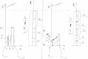
This picture indicates, among other things, that the bars become thinner and shorter at the same time, while the height-to-width ratio stays essentially constant and depends only on the location of the bar. According to Eq.1, this ratio is equal to the function $\Omega(E)$ itself:

(3) $\begin{equation*} \Omega (E) = \lim_{dE \to 0} \: \frac{d \Gamma (E)}{dE} \end{equation*}$

Note the function $\Omega$ is, thus, not only the derivative of $\Gamma$ , but also the density of states because it gives the number of states per energy interval!

(If the notation $d \Gamma (E)$ is still confusing, consider a simple function $f(x)=x^2$ . Then $df(x) \equiv d(f(x))= d(x^2)=2x \, dx$ . Consequently, $df(x)/dx \, =\, 2x$ is simply the derivative of the function $f(x)$ with respect to its argument $x$ . To obtain $d(x^2)=2x \, dx$ , we do this: $d(x^2)\equiv (x+dx)^2 - x^2 = 2x \, dx + (dx)^2$ and then drop the $(dx)^2$ term because it can be made arbitrarily smaller than the $2x \, dx$ term in the limit $dx \to 0$ .)

Once histogrammed according to their respective values of energy, the microstates lose all their identifiers other than the energy itself. Thus, two states within a single bin are no longer distinguished, in our description. In this way, the description is a reduced one. Yet this apparent sacrifice enables one to greatly simplify bookkeeping the accessible states, since now one can rewrite the discrete sum for the number of accessible states as a continuous integral:

(4) $\begin{equation*} Z \: \equiv \: \sum_i \, e^{-\beta \, E_i} \: = \: \int \, d\Gamma (E) \: e^{-\beta \, E} \: = \: \int \, dE \: \frac{d \Gamma (E)}{dE} \: e^{-\beta \, E} \: = \: \int \, dE \:\: \Omega(E) \: e^{-\beta \, E} \end{equation*}$

Note that the infinite temperature limit of $Z$ is simply the total number of states $\Gamma$ : $Z(\beta=0)=\Gamma(E_\text{max})$ , that is, all of the microstates become equally likely and, thus, automatically accessible.

Now, the integrand in Eq. (4), $\Omega(E) \, e^{-\beta \, E}$ , is clearly the probability distribution for the energy:

(5) $\begin{equation*} p(E) \, = \, \Omega(E) \, e^{-\beta \, E} \end{equation*}$

This distribution is not normalized to one, but, instead to the number of accessible states, per Eq. (4):

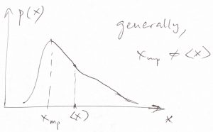
(6) $\begin{equation*} \int \, dE \, p(E) \:=\: Z \end{equation*}$

The maximum of the probability distribution $p(E)$ then determines the most probable value of the energy, a quantity of considerable interest. As illustrated in the picture below, this maximum is determined by an interplay between the rapidly increasing function $\Omega(E)$ and the rapidly decreasing function $e^{-\beta \, E}$ .

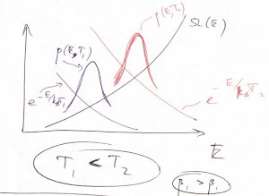
Physically, $\Omega(E)$ is an increasing function of energy because at higher energies, particles move faster and can get closer together, implying there is more available space, effectively. The decrease of the factor $e^{-\beta \, E}$ , on the other hand, apparently indicates that borrowing energy from the environment becomes harder as the temperature is lowered: The lower the temperature, the greater the $\beta$ , the faster the factor $e^{-\beta \, E}$ decays with $E$ .

We have seen that the degeneracy $\Omega(E)$ is expected to scale exponentially or faster with the system size $N$ and thus it will be convenient to introduce a new function $S(E)$ , called the entropy:

(7) $\begin{equation*} \Omega(E) \: \equiv \: \frac{1}{\delta E} \: e^{S(E)/k_B} \end{equation*}$

where we introduced a pre-exponential factor $1/\delta E$ of dimensions inverse energy to account for the fact that the quantity $\Omega$ as defined in Eq. (1) has dimensions of inverse energy. By construction, the quantity $\delta E$ depends on the system size $N$ more slowly than the exponential part $e^{S(E)/k_B}$ . According to the definition above, one may think of the entropy as the logarithm of the number of states:

(8) $\begin{equation*} S(E) \:\equiv\: k_B \ln [\Omega(E) \, \delta E] \end{equation*}$

We use the Boltzmann constant $k_B$ in the definition of entropy for historical reasons. Sometimes this historical artifact makes life more convenient and sometimes it is a nuisance, but there is no deep physics there. The entropy is, fundamentally, a dimensionless quantity which we obtain by taking the logarithm of a number. A more rigorous argument is quite obtuse and is beyond the scope of this course, but it should be immediately clear that the quantity $\delta E$ has dimensions of energy and, furthermore refers to the total energy of the system. (In fact, it reflects the magnitude of energy variations.) Thus $\delta E$ scales at most linearly with the system size $N$ or more slowly. This is much slower than the exponential dependence of $\Omega(E)$ on $N$ and so $\delta E$ can be neglected in most cases of interest. Thus, we can write:

(9) $\begin{equation*} S(E) \:=\: k_B \ln [\Omega(E) ] \end{equation*}$

while being mindful that, strictly speaking, this equation is incorrect dimensions-wise and there is an omitted additive contribution that would have restored the correct dimensions. In contradistinction with the common—also misleading and overused—notion that the entropy is a measure of disorder, it is best thought of as a measure of diversity or multiplicity of states at a given value of energy.

A remarkable feature of the entropy is that it is additive for non-interacting systems. Indeed, the total number of states for a compound system made of uncorrelated sub-systems 1 and 2 is simply the product of the respective numbers of states:

(10) $\begin{equation*} \Omega(E) \,=\, \Omega_1(E_1) \: \Omega_2(E_2) \end{equation*}$

where we should take care to note that the total energy of two non-interacting systems is the sum of the energies of the individual sub-systems:

(11) $\begin{equation*} E \:=\: E_1+E_2 \end{equation*}$

Taking the logarithm of this equation and multiplying by $k_B$ yields, in view of Eq. (9), that

(12) $\begin{equation*} S(E) \:=\: S_1(E_1) \,+\, S_2(E_2) \end{equation*}$

This equation (or its equivalent in Eq. (10) is yet another manifestation of the statistical independence of uncorrelated systems, which does not explicitly refer to specific microstates but, instead, only to their energies. Eq. (12) is thus generally distinct from the more basic equation $g(E^{(1)}_{k_1}+E^{(2)}_{k_2}) = g(E^{(1)}_{k_1}) \times g(E^{(2)}_{k_2})$ we wrote earlier for the individual contributions of microstates to the accessible number of states. No less important is the implication that according to Eq. (12), the entropy is an extensive variable, i.e. it scales linearly with the system’s size $N$ . Indeed, suppose the subsystems 1 and 2 are identical. Thus the compound system is simply twice bigger. At the same time, its entropy is twice larger than that of an individual sub-system, according to Eq. (12). For the very same reason, the energy is also an extensive quantity, see Eq. (11).

In view of the entropy’s definition, (9), we can rewrite Eq. (4) in a rather revealing form:

(13) $\begin{eqnarray*} Z &=& \int dE e^{-\beta [E - T S(E)]} \\ &\equiv& e^{-\beta \tilde{A}(E, T)} \end{eqnarray*}$

where we have defined a new, energy-like quantity:

(14) $\begin{equation*} \tilde{A}(E) \:\equiv\: E \, -\, T \, S(E) \end{equation*}$

and we keep in mind, that in addition to the energy $E$ , the function $\tilde{A}(E)$ also depends on the temperature $T$ , volume, the particle number, and, possibly, other quantities.

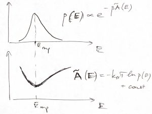
Now the probability distribution for energy values can now be written in a rather simple fashion:

(15) $\begin{equation*} p(E) \:\propto\: e^{-\beta \tilde{A}(E)} \end{equation*}$

Because the function $e^{-x}$ is a monotonically decreasing function of its argument, the maximum of the probability $e^{-\beta \tilde{A}(E)}$ is located exactly at the minimum $E_\text{mp}$ of the function $\tilde{A}(E)$ . Thus the problem of finding the likeliest value of the energy, at some fixed value of temperature and volume, etc., is reduced to finding the minimum of the energy-like quantity $\tilde{A}(E)$ .

Furthermore, after comparing the quantity $e^{-\beta \tilde{A}(E)}$ with the Boltzmann distribution for a particle subject to a potential energy ${\cal V}(x)$ :

(16) $\begin{equation*} p(x) \:\propto\: e^{-\beta \, {\cal V}(x)} \end{equation*}$

we conclude that the function $\tilde{A}(E)$ plays the role of a potential energy for the energy of the system itself! (Isn’t that fascinating?) For this reason, it can be called a thermodynamic potential. Furthermore, the most probable value of the energy corresponds with the equilibrium position of the thermodynamic potential $\tilde{A}(E)$ . Thus we have a license to vividly think of thermodynamic equilibrium as a mechanical equilibrium with respect to thermodynamic potentials. We will see soon, that similar thermodynamic potentials can be written down for other important thermodynamic quantities such as the volume or the chemical composition of a reactive mixture. The possibility of writing such thermodynamic potentials for quantities of interest is, arguably, the most important outcome of Thermodynamics. Note that those quantities are not even dynamical variables! But it gets even more interesting from here.

By how much should we expect the energy to fluctuate around its most likely value? Let us Taylor expand our thermodynamic potential around $E_\text{mp}$ up to the second order in deviation of the energy from its most probable value $E_\text{mp}$ :

(17) $\begin{eqnarray*} \tilde{A}(E) &\approx& \tilde{A}(E_\text{mp}) + \left. \frac{\partial \tilde{A}}{\partial E} \right|_{E=E_\text{mp}} (E- E_\text{mp}) + \frac{1}{2} \left. \frac{\partial^2 \tilde{A}}{\partial E^2} \right|_{E=E_\text{mp}} (E- E_\text{mp})^2 \\ &=& \tilde{A}(E_\text{mp}) + \frac{1}{2} \left. \frac{\partial^2 \tilde{A}}{\partial E^2} \right|_{E=E_\text{mp}} (E- E_\text{mp})^2 \end{eqnarray*}$

where in the 2nd equation we took account of the fact that the first derivative of a function vanishes at a minimum: $\left. \frac{\partial \tilde{A}}{\partial E} \right|_{E=E_\text{mp}} = 0$ . We recall that the Taylor expansion is a way to approximate complicated functions using a relatively simple functional form, i.e, a polynomial. The narrower the involved interval of the argument, the lower order polynomial is needed to achieve a given accuracy. By construction, discarding terms of order $(E- E_\text{mp})^3$ and higher implies that we are approximating our function by a parabola.

Substituting Eq. (17) into Eq. (15) yields

(18) $\begin{equation*} p(E) \:\approx \: \frac{1}{\delta E} e^{-\beta \tilde{A}(E_\text{mp})} \:\: e^{- \frac{\beta}{2} \left. \frac{\partial^2 \tilde{A}}{\partial E^2} \right|_{E=E_\text{mp}} (E- E_\text{mp})^2 } \end{equation*}$

This, then, shows that the probability distribution of the energy is a Gaussian distribution where, we see, the variance is proportional to the inverse 2nd derivative of $\tilde{A}(E)$ at the minimum:

(19) $\begin{equation*} \sigma^2 \:=\: \left( \frac{\beta \: \partial^2 \tilde{A}}{\partial E^2} \right)_{E=E_\text{mp}}^{-1} \end{equation*}$

Let us focus, for a moment, on the scaling of the variance of the energy distribution with the system size $N$ . We already noted that the energy scales linearly with the system size thus allowing one to define the energy per particle $\varepsilon \equiv E/N$ , which is an intensive variable that carries no information whatsoever about the system size. Thus,

(20) $\begin{equation*} E \:=\: N \, \varepsilon \end{equation*}$

Likewise, we can define the intensive analog of the quantity $\tilde{A}$ :

(21) $\begin{equation*} \tilde{A} \:=\: N \, \tilde{a} \end{equation*}$

because $\tilde{A}$ is an extensive quantity, being the sum of two extensive quantities: $E$ and $-TS(E)$ . Hence we infer that the variance of the energy scales linearly with the system size:

(22) $\begin{equation*} \sigma^2 \:=\: \left( \frac{\partial^2 \tilde{A}}{\partial E^2} \right)_{E=E_\text{mp}}^{-1} \:=\: N \, \left( \frac{\partial^2 \tilde{a}}{\partial \varepsilon^2} \right)_{\varepsilon=\varepsilon_\text{mp}}^{-1} \end{equation*}$

This is an incredibly important result because it shows that the rmsd of the energy from its most probable value scales only as a square root of the system size:

(23) $\begin{equation*} \delta E = \sigma \:\propto\: \sqrt{N} \end{equation*}$

Consequently, the relative magnitude of the energy fluctuation scales inversely with $\sqrt{N}$ and, thus, can be made arbitrarily small given a sufficiently large system:

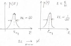
(24) $\begin{equation*} \frac{\delta E}{E_\text{mp}} \:\propto\: \frac{1}{\sqrt{N}} \end{equation*}$

Thus we observe that in a practically important limit of large systems— $N$ could be as large as $10^{23}$ —the probabilistic description above becomes essentially deterministic, since the intensive properties become sharply defined. To put this in perspective, let us estimate the chances that the energy per particle deviates, say, by 0.001%=10^-5 from its most probable value for a system containing one mole of particles. Typically, $\varepsilon \sim k_B T$ , up to a numerical factor of order one. We will learn soon that $(\partial^2 \tilde{A}/\partial E^2)^{-1} = C_V T$ , where $C_V$ is the heat capacity at fixed volume. This means that at constant volume, $\delta E = \sqrt{C_V k_B T^2}$ . The heat capacity is typically $k_B$ or less, per particle. Thus the reduction in the probability, off its largest value, is $e^{-(E-E_\text{mp})^2/2 (\delta E)^2} \sim e^{- N (\varepsilon-\varepsilon_\text{mp})^2/2 (C_V/N)} k_B T^2} = e^{-6 \times 10^{23} \times (10^{-5})^2/2} = e^{-3 \times 10^{13}} \sim 10^{-10^{13}}$ , a monstrously small number that has $10^{13}$ zeros, or so, after the decimal point. Conversely, if you happened to witness such a deviation, your chances of observing it again are essentially zero. There are important consequences of this rapid falloff in the probability:

If a very large system happens to be in equilibrium, which minimizes the pertinent thermodynamic potential, it will remain in equilibrium. (The precise identity of the thermodynamic potential depends on the specifics of the experiment and will be discussed as we proceed.) Conversely, if the system happens to be away from equilibrium—for instance, because we had temporarily imposed a constraint and then let go—it will spontaneously and irreversibly evolve toward equilibrium, so as to minimize the pertinent thermodynamic potential, and then, again, will stay there forever. This is the essence of the 2nd Law of Thermodynamics, which essentially says that the most probable process will occur with probability one.
For systems that are not too large, fluctuations of thermodynamic variables off their most likely values are noticeable, however, are usually small. Since the quadratic expansion of thermodynamic potentials, such as that in Eq. (17), approximates the potential well in a small range, the statistics of thermodynamical variables are subject to the Gaussian distributions. The maximum of the distribution is located at the minimum of the corresponding thermodynamic potential, as in Eq. (17). The width of the distribution is determined by curvature (2nd derivative) of the thermodynamic potential, as in Eq. (19).
Because the most probable value and the average value for the Gaussian distribution coincide, we conclude that the expectation value of a thermodynamic variable corresponds to its equilibrium value, i.e, the value that minimizes the corresponding thermodynamic potential. This is not simply a formal remark. On the contrary, the mean and the most probable value of a distribution are generally not equal to each other (though often are numerically close), see Figure below. Thus in the rest of the Thermo part of the Course, we will use the terms “average” and “most probable” interchangeably, while being mindful that it is the average, i.e., expectation value of a quantity that is measured in an experiment.

That the fluctuations of extensive quantities should scale with $\sqrt{N}$ is as important as it is somewhat nonintuitive. Indeed, why should it be that a quantity whose value is so large, i.e., proportional to the particle number $N$ itself, should have fluctuations that are much smaller? The answer to this is that in a sufficiently large system, separate parts behave sufficiently independently so that their fluctuations are not correlated and, hence, will largely cancel out when added together.

Let us now write out a necessary condition for the minimum of the thermodynamic potential $\tilde{A}$ , where it is understood that $\tilde{A}$ is a function of three variables: $E$ , $T$ , and $V$ , and we are keeping the temperature and volume constant:

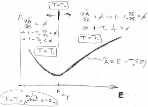
(25) $\begin{equation*} \frac{\partial}{\partial E} \tilde{A} \:=\: \left. \frac{\partial}{\partial E} [E - T\, S(E, V) ] \right|_{E=E_\text{mp}} \:=\: 1 - T\, \left. \left( \frac{\partial S}{\partial E} \right)_V \right|_{E=E_\text{mp}} \:=\: 0 \end{equation*}$

The explicit volume dependence of $\tilde{A}$ is exclusively through the entropy, $S=S(E, V)$ , which we have indicated. Since the minimum of $\tilde{A}$ corresponds with equilibrium, the above equation yields that the equilibrium value of the energy and the temperature are not independent but, instead, inter-relate via the following constraint:

(26) $\begin{equation*} \left. \left( \frac{\partial S}{\partial E} \right)_V \right|_{E=E_\text{mp}} \:=\: \frac{1}{T} \end{equation*}$

Here we also explicitly indicate that the volume is being kept constant. Because of this dependence, we use the partial derivative with respect to $E$ in Eq. (26). This equation can interpreted in, essentially, two ways. On the one hand, suppose we know that our system is, in fact, equilibrated while being at a certain value of energy $E_0$ . Then, Eq. (26) tells us that the temperature must be equal to the derivative $\frac{\partial S}{\partial E}$ taken exactly at point $E=E_0$ . In this way of doing things, the temperature $T$ is a function of the expectation value of the energy:

(It is also a function of volume $V$ , because the entropy $S$ is a function of both $E$ and $V$ .) On the other hand, suppose we bring our system in contact with a much larger system whose temperature is $T_0$ . What happens if the system’s is energy is, say, lower than its equilibrium value? Then $\partial \tilde{A}/\partial E < 0$ , which implies $1 - T_0 (\partial S/\partial E) < 0$ or, by virtue of Eq. (26), that $T < T_0$ . This is consistent with the definition of temperature! Indeed, since the volume and particle number are kept constant, the only way for the system to receive energy is via heat exchange. Thus the inequality $T < T_0$ is consistent with fact that the heat will flow to the system so as to enable it to increase its energy until it reaches its equilibrium value, at which point $T=T_0$ .

The case of the system’s having initially a higher than the equilibrium value of energy is entirely analogous.

In contrast with independent variable $E$ , the equilibrium value of the energy is constrained by Eq. (26) and is now a function of temperature $T$ an volume $V$ :

(27) $\begin{equation*} E_\text{mp} \:=\: E_\text{mp}(T, V) \end{equation*}$

The same applies to the equilibrium value of entropy:

(28) $\begin{equation*} S(T, V) \:=\: S[ E_\text{mp}(T, V), V] \end{equation*}$

where we recapitulated that the entropy $S=S(E, V)$ from Eq. (7) may depend on the volume explicitly, and now, also through $E_\text{mp}(T, V)$ .

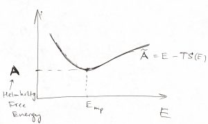
Now, note that the equilibrium value of the function $\tilde{A}$ is, in fact, is the minimum value of $\tilde{A}$ . We now define the the Helmholtz free energy as this equilibrium, minimum value of $\tilde{A}$ :

We reiterate that the quantity $\tilde{A}$ is a function of three variables, i.e., $E$ , $V$ , $T$ . In contrast, the Helmholtz free energy is a function of only two independent variables, because of the constraint imposed by Eq. (26), which thus eliminates one degree of freedom. By virtue of Eqs. (27) and (28), a natural (but not unique) choice of those two independent variables is temperature and volume:

(29) $\begin{equation*} A(T, V) \:\equiv \: \tilde{A}(E_\text{mp}(T, V), T, V) \: = \: E_\text{mp}(T, V) - T S[E_\text{mp}(T,V), V]\end{equation*}$

where we used Eq. 14. From this moment on, we will consider exclusively equilibrium configurations. To simplify notations, we will drop the “mp” label:

(30) $\begin{equation*} E_\text{mp} \: \to \: E \end{equation*}$

It is also worthwhile to streamline Eq. (29)

(31) $\begin{equation*} A \: \equiv \: E - TS \end{equation*}$

Now consider a small increment of both sides of Eq. (31):

(32) $\begin{equation*} (dA)_V \:=\: (dE)_V - d(TS)_V \:=\: (dE)_V - [S(dT)_V+T(dS)_V] \end{equation*}$

where, in the usual way, we retain only quantities that are first order in the increment and discard higher order terms because they can be made arbitrarily smaller by decreasing the magnitude of the increment: $d (x y) \equiv (x+dx)(y+dy)- xy = xdy + ydx + dx dy \approx xdy + ydx$ .

Eq. (32) can be greatly simplified after we recall that the temperature can be regarded as a function of the equilibrium value of the energy: $E=E_\text{mp}(T) \Rightarrow T=T(E)$ or, equivalently, of the equilibrium value of the entropy, see the Figure following Eq. (26). It is, then, convenient to re-write Eq. (26) here in an equivalent form:

(33) $\begin{equation*} T \:=\: \left(\frac{\partial E}{\partial S}\right)_V \end{equation*}$

This way, $E$ and $T$ are regarded as functions of the variables $S$ and $V$ and we are varying the variable $S$ , in Eq. (33), while keeping the volume $V$ constant.

One can rewrite Eq. (33) profitably as

(34) $\begin{equation*} (dE)_V \:=\: T dS \end{equation*}$

which says that the energy increment in a slow isochoric process is simply the entropy increment times the temperature. (“Isochoric”=”taking place at constant volume”.) The reason we must specify that the process be slow is that past Eq. (29), we have limited ourselves to processes where the energy (and all other quantities) are at their equilibrium values.

Eqs. (33) and (32) then readily yield

(35) $\begin{equation*} (dA)_V \:=\: -S (dT)_V \text{ or, equivalently, } S \:=\: -\left(\frac{\partial A}{\partial T}\right)_V \end{equation*}$

We have seen that the free energy is extremely useful as its value is directly tied to the probability of the corresponding thermodynamic state. Yet the entropy $S$ , the energy $E$ , and the Helmholtz free energy $A$ are not directly measured in experiment. Let us, then, further elaborate on the physical meaning of these thermodynamic functions and the implications of the present formalism for experiment. To do so, we will invoke a physical law while also explicitly considering changes in the volume. The physical law in question is the law of conservation of energy. In the present context, this law states that changes in the system’s energy, if any, can result from either heat exchange or work performed by the system:

(36) $\begin{equation*} dE \:=\: \delta Q \:-\: \delta W \hspace{5mm} \leftarrow \text{ "The 1st Law" } \end{equation*}$

where $\delta Q$ is the amount of heat the system has received or given up during the process in question, while $\delta W$ is the work performed by the system. It suffices to note for now that the symbols $d$ and $\delta$ indicate that we are considering small amounts; their precise meaning will be clarified later. As stated above, the law of conservation of energy is referred to as the First Law of Thermodynamics.

As already alluded to in Chapter 2, breaking up the full energy change into contributions due to heat exchange and work, respectively, is empirical and, admittedly, somewhat artificial. Informally speaking, we divide the processes behind the energy/momentum exchange between our system and its environment into those processes that we cannot directly see or control (heat exchange) and those that we can, in fact, directly see and control (work). This way of doing things was inevitable in the early days, when advanced microscopy was unavailable, but remains increadibly useful to this day and will remain so for the foreseeable future; we can “see” a lot more these days but individually controlling huge numbers of degrees of freedom will remain impossible. In any event, because of the empirical nature of Eq. (36), we should remain careful. For instance, if one want to consider work in the absence of heat exchange, one must remember that there is no perfect way to thermally insulate a system and so a $\delta Q=0$ process is an idealization that is adequate on short enough times scales such that relatively little heat exchange has occurred. On the other hand, those short times should still be longer than the relaxation time of the system, if we want to use results developed under the assumption of equilibrium. This is rarely a problem in practice, since mechanical equilibration often occurs on time scales that are shorter than characteristic times of heat exchange, a notable exception represented by convection processes, such as those leading to hurricanes.

Above said, let us write down an expression for the performed work. According to the picture below:

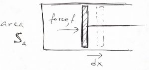
one can evaluate the work done by the system as

(37) $\begin{equation*} \delta W \:=\: f \: dx \:=\: \frac{f}{S_a} \: S_a dx \:=\: p \, dV \end{equation*}$

where $p=f/S_a$ is our old friend pressure, not probability (!). A more general argument that applies to arbitrary geometries can be found in the CHEM4370 notes. In addition to providing an explicit expression for the work, the above equation shows that no work is performed if there are no volume changes, something we already new. Thus we obtain

(38) $\begin{equation*} (dE)_V \:=\: \delta Q \end{equation*}$

a statement made without explicit reference to the time scale of the experiment. We now compare this equation with Eq. (34), which was written for slow processes, and notice that the right hand sides of the two equations do not contain an explicit reference to whether the process is isochoric or not and, thus, should be equal to each other under general circumstances, so long as the conditions for the individual equations are met. Thus we obtain that for slow processes, such that the system can be regarded as equilibrated at any given time, there is one-to-one correspondence between heat exchange and entropy changes:

(39) $\begin{equation*} \delta Q \:=\: T dS \end{equation*}$

A somewhat less Jesuitical way to show that Eq. (39) applies to arbitrary non-isochoric processes connecting two states with different volumes, we note that any process, in which the entropy and volume are changing at the same time, can be always thought of as a step-like process of the kind depicted below:

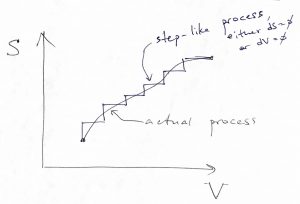
This is because in equilibrium, the energy can be regarded as a function of two variables and so the energy increment $\Delta E = E_\text{final} - E_\text{initial}$ resulting from a change in those variables is not affected by the shape of the path connecting the initial and final state of the process, but only on the values of those variables at the end-points of the path. For the same reason, the change in the altitude resulting from traveling from one town to another will be the same no matter which route the traveler used. The energy is what they call a state function. (There is a third variable, the particle number $N$ , but we are keeping it constant throughout this Chapter.) Next notice that entropy changes will be collected only along those legs of the process where the volume stays constant where no work is being done and thus only heat is being exchanged between the system and its environment. By taking the limit of an infinitely small step size, we can make the values of any quantity, such as the temperature or pressure etc., along the jagged path to be arbitrarily close to that for the actual, smooth path. Conversely, we will see in due time that heat and work are not state functions, hence our using $\delta$ , not $d$ in Eq. (36).

Eq. (39) drives home the statistical foundation of Thermodynamics. On the one hand, entropy reflects the number of degrees of freedom that we chose not to control or could not control in principle. On the other hand, that heat has to do precisely with molecular motions, which we cannot control individually in principle. We can only control some of the average characteristics of those motions, such as the average kinetic energy.

Thus we obtain that for slow, or quasistatic processes such that the system can be regarded as equilibrated at all times:

(40) $\begin{equation*} dE \:=\: T dS \:-\: p \, dV \end{equation*}$

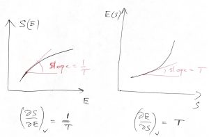
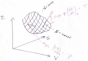
In other words, if during some (elemental) slow process, the entropy underwent a change $dS$ and volume $dV$ , then one can immediately evaluate the resulting change in the energy, if the temperature and pressure are known. In fact, the temperature specifies the rate of change of energy with entropy at constant volume, while the negative pressure specifies the rate of change of energy with volume at constant entropy:

(41) $\begin{align*} T &= \left(\frac{\partial E}{\partial S}\right)_V \\ -p &= \left(\frac{\partial E}{\partial V}\right)_S \end{align*}$

Indeed, the top equation is obtained by setting $dV=0$ ( $V=\text{const})$ in Eq. (40) and dividing by $dS$ , while the top equation is obtained by setting $dS=0$ ( $S=\text{const})$ and dividing by $dV$ . This can be illustrated graphically:

Eq. (40) may well be the most consequential equation of the Course, as far as its quantitative implications are concerned. (The equation will be later generalized to cases when we allow the particle number to change, as would be necessary, for instance, in Thermochemistry.) The first thing to do is to obtain a differential of the Helmholtz free energy $A\equiv E-TS$ :

(42) $\begin{equation*} dA \:=\: d(E-TS) \:=\: dE -T dS -SdT \end{equation*}$

which, by virtue of Eq. (40), leads to a simple result:

(43) $\begin{equation*} dA \:=\: -SdT \:-\: p \, dV \end{equation*}$

or, equivalently,

(44) $\begin{align*} -S &= \left(\frac{\partial A}{\partial T}\right)_V \\ -p &= \left(\frac{\partial A}{\partial V}\right)_T \end{align*}$

What is is the significance and use of Eqs. (41) and (44) for practical applications? In the ideal turn of events, one can calculate the density of states $\Omega(E, V)$ and, thus, evaluate $S(E, V) = k_B \ln \Omega(E, V)$ . One then solves this for the energy as a function of entropy and volume $E=E(S, V)$ . Next, one uses Eq. (41) to calculate the temperature and pressure as functions of entropy and volume: $T=T(S, V)$ and $p=p(S, V)$ . Now we have four quantities— $T$ , $S$ , $p$ , and $V$ —and two equations connecting them, implying only two of those quantities are independent. This means that we can predict, in principle, the pressure as a function of volume and temperature and thus predict the equation of state: $p=p(V, T)$ . To be clear, the dependences $V=V(p, T)$ and $T=T(V, p)$ are also called equations of state. Given the $p(V, T)$ dependence is known, one can then calculate important response functions, such as the isothermal compressibility:

(45) $\begin{equation*} \kappa_T = - \frac{1}{V} \left( \frac{\partial V}{\partial p} \right)_T \hspace{8mm}\leftarrow \text{ isothermal compressibility}\end{equation*}$

or its inverse, called the bulk modulus

(46) $\begin{equation*} \kappa_T = - V \left( \frac{\partial p}{\partial V} \right)_T \hspace{8mm}\leftarrow \text{ bulk modulus}\end{equation*}$

These quantities are of utmost importance in materials science as they reflect how compressible/stiff the material is. Note the factors in front of the derivatives are needed to make these important response functions intensive quantities. In other words, we are talking about relative, not absolute volume changes. Another important response function is the thermal expansion coefficient:

(47) $\begin{equation*} \alpha = \frac{1}{V} \left( \frac{\partial V}{\partial T} \right)_p \hspace{8mm} \leftarrow \text{ thermal expansivity}\end{equation*}$

which tells one how much the object will expand or contract as the temperature changes. For instance, chemical glassware is made of quartz, not ordinary window glass because the latter has too large an expansion coefficient. As a result, washing a hot beaker with cold water would create large strains and result in its breaking.

If, on the other hand, one uses the relations $T=T(S, V)$ and $p=p(S, V)$ to express the entropy as a function of temperature and volume: $S=S(T, V)$ , one can readily evaluate the heat capacity at constant volume:

(48) $\begin{equation*} C_V \equiv \left( \frac{\delta Q}{\partial T} \right)_V = T\left( \frac{\partial S}{\partial T} \right)_V \hspace{8mm}\leftarrow \text{ heat capacity at constant volume}\end{equation*}$

and, likewise, the heat capacity at constant pressure:

(49) $\begin{equation*} C_p \equiv \left( \frac{\delta Q}{\partial T} \right)_p = T\left( \frac{\partial S}{\partial T} \right)_p \hspace{8mm}\leftarrow \text{ heat capacity at constant pressure}\end{equation*}$

Alternatively, if one can evaluate the Helmholtz free energy as a function of temperature and volume, $A=A(V, T)$ , one may infer the entropy and pressure using Eq. (44) and follow the rest of the program as just described. In practice, it is often mathematically easier to go the Helmholtz route, which is called the “canonical” formalism. (The $S(E)$ centered formalism is often referred to as “microcanonical”.) The key notion here is that after one substitutes the Gaussian approximation for the probability density (18) into Eq. (6) and integrates, one obtains: $Z=\frac{\sqrt{2 \pi \sigma^2}}{\delta E} \, e^{-\beta A}$ , where used Eq. (29). The pre-exponential factor scales only algebraically, i.e. as a power, with the system size, while the exponential scales exponentially, which is a much much faster dependence. Thus, to a leading order in $N$ , the Helmholtz energy is related to the partition function $Z$ in a very simple way:

(50) $\begin{equation*} Z\:=\:e^{-\beta A} \end{equation*}$

or

(51) $\begin{equation*} A \:=\: -k_B T \ln Z \end{equation*}$

An interesting corollary of Eq. (50) is that if the system has more than one stable or metastable states and so one can define a Helmholtz free energy for each minimum, as in the Figure below:

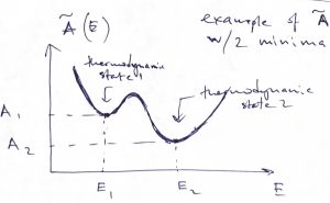
then the probability of being in the thermodynamic state 1 relative to the thermodynamic state 2 is simply the exponential of the free energy difference times $(-\beta)$ :

(52) $\begin{equation*} \frac{Z_1}{Z_2} \:=\:\frac{e^{-\beta A_1}}{e^{-\beta A_2}} \:=\: e^{-\beta (A_1-A_2)} \end{equation*}$

We reiterate that each of the thermodynamic states 1 and 2 is generally a vast ensemble of microstates characterized by some value of energy. The number of accessible microstates is given by the quantity $Z$ . The probability ratio for two distinct thermodynamic states is given by the ratio of the respective numbers of the states accessed by the system, hence Eq. 52. After we compare the result in Eq. 52 to the probability ratio of two microstates: $p_1/p_2=e^{-\beta(E_1-E_2)}$ , we conclude that when one cannot control the identity of the microstate, but can only control the average value of the energy—by bringing the system in contact with an environment—the relevant probabilities are determined not by the energy itself but, instead, by the free energy. Often, what we regard as distinct “thermodynamic states” refer to distinct phases or physical states with distinct properties, such as a folded and unfolded protein molecule, respectiveliy. In view of Eq. (31), the probability ratio from Eq. 52 becomes

(53) $\begin{equation*} \frac{Z_1}{Z_2} \:=\:\frac{e^{S(E_1)/k_B}}{e^{S(E_2)/k_B}} e^{-\beta (E_1-E_2)} \:=\: \frac{\Omega(E_1)}{\Omega(E_2)} \: e^{-\beta (E_1-E_2)} \end{equation*}$

i.e., in the presence of multiplicity of microstates at a particular value of energy, the distribution of energy is determined by that multiplicity, in addition to the Boltzmann weight $e^{-\beta E}$ , as we saw already in the last Chapter. We have now generalized those early ideas to apply to rather arbitrary structures of energy levels. Per Eq. 52, two thermodynamic states are equally likely, at fixed volume and temperature, when their Helmholtz energies are mutually equal:

(54) $\begin{equation*} A_1 \:=\: A_2 \text{ for two states in equilibrium} \end{equation*}$

which, then, provides a criterion for things like the folding transition of a protein. In turn, this means

(55) $\begin{equation*}E_1 - T S_1 \:=\: E_2 - T S_2 \end{equation*}$

We observe an important pattern: If one state is stabilized in terms of energy, then the other state should have a higher entropy.

Note that per Eq. (31), the energy and free energy become equal at $T=0$ , i.e. when the molecular motions stop. These are the motions that are responsible for the degeneracy, in the first place. Accordingly, $A=E$ at any temperature, if the energy levels are non-degenerate, $S=0$ , i.e., there are no degrees of freedom we are not explicitly controlling.

Why the free energy? We can integrate Eq. (40) at constant entropy ( $S=\text{const}$ , $dS=0$ ), to see that the work performed by the system in the absence of heat exchange is given by the decrease in the energy:

(56) $\begin{equation*} \Delta E_S \:=\: \int_1^2 (dE)_S \:=\: - \int_1^2 p \, dV \end{equation*}$

This is analogous to our earlier statement that the work of a conservative force is the negative of the change of the potential:

(57) $\begin{equation*} \Delta {\cal V} \:=\: \int_1^2 d {\cal V} \:=\: - \int_1^2 f \, dx \end{equation*}$

In contrast, integration of Eq. 43 at constant temperature ( $T=\text{const}$ , $dT=0$ ) shows that the work performed by the system that exchanges heat with the environment, so as to maintain its temperature, is given by the decrease in the free energy:

(58) $\begin{equation*} \Delta A_T \:=\: \int_1^2 (dA)_T \:=\: - \int_1^2 p \, dV \end{equation*}$

Again, note the formal similarity of this statement with how the decrease in the potential energy relates to the work of a conservative force, per Eq. (57). This similarity provides yet another justification for the term “thermodynamic potential”. In any event, we see the word “free” in the term “free energy” refers to energy available to do useful work. In contrast with the case from Eq. 56, the energy comes not only from the system itself, but also from the environment. Indeed, given the same amount performed work in Eqs. 56 and 58, respectively, the energy decrease in the latter case is smaller than in the former case: First we note that since $\Delta A_T=\Delta(E-T S)_T = \Delta E - T \Delta S_T$ , we can write $\Delta E_T = \Delta A_T + T \Delta S_T = \Delta E_S + T \Delta S_T$ . The system performs useful work only when it expands, so that $pdV > 0$ . At the same time, an increase in volume at constant temperature implies an increase in the entropy. Hence, $T \Delta S_T > 0$ and, consequently, $\Delta E_T > \Delta E_S$ , where note both quantities are negative. Thus we conclude that if the system exchanges heat with environment—so as to keep its temperature steady—the amount of useful work the system can perform at its own expense is lowered. To extract the same amount of work as in the $\Delta S=0$ case, one must supply heat from the outside. Informally speaking, the amount of useful work extracted from the system proper is lowered because the system is “holding on” to the thermal portion of its internal energy when the temperature is held constant. Conversely, to compress a system isothermally, one needs to extract heat from it. The latter notion will be useful later on, when we discuss thermal engines. There, we shall see that an engine cycle must contain portions that correspond to isothermal compression. Because the latter process requires outflow of heat—which is ordinarily not recycled—the efficiency of the engine is lowered.

Now, the number of accessible states $Z=Z(T, V)$ , which is an explicit function of temperature and volume, is usually (but not always!) easier to compute than $S=S(E, V)$ . For this reason, the canonical formalism is often preferred for calculations. Yet a quality evaluation of $Z$ from scratch is often hard, too. But sometimes, the equation of state and calorimetric data are already known, for instance from experiment. (Calorimetry has to do with measuring the heat capacity.) It is then possible to extract the free energy from that information and other quantities of interest using the present description as a formal framework. We will illustrate this hybrid approach here for the ideal gas, since we do happen to know its equation of state:

(59) $\begin{equation*} p V = N k_B T \end{equation*}$

Since we do not have—as of yet—an expression for the entropy, neither of the equations (41) and (44) suffice to determine the free energy. However, we do have some access to the calorimetry since we know the temperature dependence of the energy. It is simply the number of particles times $k_B T/2$ times the number of degrees of freedom $n_\text{d.o.f.}$ :

(60) $\begin{equation*} E \:=\: N \frac{k_B T}{2} n_\text{d.o.f.} \end{equation*}$

We can express this through the standard heat capacity, by first setting $dV=0$ in Eqs. (40), then dividing the resulting equation by $dT$ and using Eq. (48). This yields

(61) $\begin{equation*} C_V \:=\: \left( \frac{\partial E}{\partial T} \right)_V \end{equation*}$

Differentiating Eq. (60) with respect to temperature, then, yields the following expression the heat capacity at constant volume, per particle:

(62) $\begin{equation*} c_V \:=\: \frac{C_V}{N} \:=\: \frac{k_B}{2} n_\text{d.o.f.} \end{equation*}$

while the energy of the gas can expressed through the heat capacity and temperature according to:

(63) $\begin{equation*} E \:=\: C_V T \:\equiv\: N c_v T \end{equation*}$

The full heat capacity is a sum of three contributions: translational, rotational, and vibrational. Here is a table that summarizes these three contributions:

$c_V$

translation, 3D

$\frac{3k_B}{2}$

rotation

atom	0
linear molecule	$k_B$
molecule, not linear	$\frac{3k_B}{2}$

vibration, per themally active degree of freedom, $k_B T > \hbar \omega$

$k_B$

To obtain an actual expression for the entropy as a function of temperature and volume, we first re-write Eq. (40)

(64) $\begin{equation*} dS \:=\: \frac{1}{T} dE \:+\: \frac{p}{T} \, dV \end{equation*}$

and then substitute $dE = C_V dT$ , as obtained by taking an increment of Eq. (60), and $\frac{p}{T}=\frac{N k_B}{V}$ , per the equation of state of the ideal gas:

(65) $\begin{equation*} dS \:=\: C_V \frac{dT}{T} \:+\: N k_B \, \frac{dV}{V} \end{equation*}$

This expression is very easy to integrate between any two states characterized by distinct values of the two variables, $T$ and $V$ , because they enter in the r.h.s. separately. Let’s take for the initial and final states for the integration, respectively, some standard reference state, labeled using the superscript “ $\ominus$ ” and the state at the actual temperature and volume:

(66) $\begin{equation*} S(T, V) - S(T^\ominus, V^\ominus) \:=\:C_V \ln\left(\frac{T}{T^\ominus}\right) \:+\:N k_B \ln\left(\frac{V}{V^\ominus}\right) \end{equation*}$

Note the result of the integration is expressly independent of the integration path, consistent with the the entropy being a state function. We will not proceed with explicitly calculating the Helmholtz free energy quite yet (which one could accomplish using Eq. 43) as the knowledge of the entropy will suffice for now.

We now return to the 2nd Law of Thermodynamics. We have seen that for a large system, the likeliest set of configurations will be realized with, essentially, probability 1. We have also seen that the notion of maximizing the probability, a statistical concept, is interchangeable with the notion of minimizing an appropriate thermodynamic potential, a mechanical notion. Specifically, when the volume and temperature are fixed, the equilibrium energy value is determined by the minimum of the function

(67) $\begin{equation*} \tilde{A}(E, V, T) \:\equiv\: E \, -\, T \, S(E, V) \end{equation*}$

Conversely, any configuration other than that minimizing the function $\tilde{A}(E, V, T)$ would not be equilibrium. To create such a configuration, one would have to impose some additional constraints. Such additional constraints, by definition, imply that the number of accessible configurations at a given value of $E$ is now decreased. This effectively means a smaller value of $S(E, V) \: = \: k_B \, \ln \Omega(E, V)$ and a larger value of $\tilde{A}$ , by Eq. 67. Thus one can formulate the 2nd law of Thermodynamics in the following ways:

The entropy of a large, isolated system can only increase, and cannot decrease over time. It reaches its maximum value in equilibrium.
At constant volume and temperature, the Helmholtz free energy of a large system can only decrease, and cannot increase. It reaches its minimum value in equilibrium.

A word on thermodynamic stability. The constraint (26) on the equilibrium values of energy and temperature only guarantees that the function $\tilde{A}$ —or the probability distribution $p(E)$ —is at its extremum. But we actually want a maximum for $p(E)$ and, hence, a minimum for $\tilde{A}$ . It is thus required that the second derivative of $\tilde{A}$ at $E=E_\text{mp}$ be positive. This way the extremum will be a stable minimum, not an unstable maximum or a configuration in neutral equilibrium. Therefore we must require that

(68) $\begin{equation*} \left. \frac{\partial^2 \tilde{A}}{\partial E^2} \right|_{E=E_\text{mp}} \: > \: 0 \end{equation*}$

where, note, $T$ and $V$ are kept constant. In view of Eq. 14 and the fact that $T \equiv 3 \langle m v^2/2 \rangle /k_B >0$ , this condition yields

(69) $\begin{equation*} \left( \frac{\partial^2 S}{\partial E^2} \right)_V \: < \: 0 \text{, at } E=E_\text{mp} \end{equation*}$

and note that $S(E)$ in this equation is a function of $E$ and $V$ only. We have seen, however, that the derivative $(\partial S/\partial E)_V$ at any value of $E$ is equal to the inverse temperature at that same value of $E$ , and so

(70) $\begin{equation*}\left( \frac{\partial^2 S}{\partial E^2} \right)_V \: \equiv \: \left( \frac{\partial (\partial S/\partial E)_V}{\partial E} \right)_V \: = \: \left( \frac{\partial (1/T)}{\partial E} \right)_V \: = \: - \frac{1}{T^2} \left( \frac{\partial T}{\partial E} \right)_V \: = \: - \frac{1}{C_V T^2} \end{equation*}$

where we used the chain rule of differentiation and that $d(1/T)/dT = - 1/T^2$ , and also Eq. 61. Thus we obtain a stability condition for thermal fluctuations:

(71) $\begin{equation*} C_V \: > \: 0 \end{equation*}$

It is easy to convince ourselves that if this condition is not satisfied, we would have an instability on our hands. Indeed, a negative heat capacity would imply a maximum in the $\tilde{A}$ function, which, in turn, would lead to an absurd situation: As the energy of the system becomes increasingly less than the “equilibrium” value at the extremum of $\tilde{A}$ , its temperature increases which lead to the system giving away the energy and a further decrease in the energy. This is a case of an effective force that is not restoring, but, on the contrary, pushes one away from the equilibrium point. This corresponds to an unstable equilibrium, of course.

We conclude by stating the 3rd Law of Thermodynamics. It states that the entropy must vanish at zero temperature:

(72) $\begin{equation*} S(T=0) \: = \: 0 \end{equation*}$

This law is obeyed by most systems for reasons that will become more clear in the Quantum part of the Course. Here we only note that owing to Eqs. 61 and 71, the energy must be a monotonically increasing function of temperature. Thus the energy reaches its minimum value at $T=0$ . The 3rd law, then, essentially implies that the ground state of a physical system is not degenerate, i.e., $\Omega=e^{N^\alpha}$ , where $\alpha < 1$ . And so the entropy per particle, $\frac{S}{N}= \frac{\ln \Omega}{N} = N^{\alpha-1}$ vanishes in the infinite system limit $N \to \infty$ . There are a few seeming counterexamples to the 3rd Law, but most physical systems of interest in this Course do obey this law. In turn, it provides for a helpful (though not mandatory) way to define a standard state for the entropy.

License

Icon for the Creative Commons Attribution-NonCommercial-NoDerivatives 4.0 International License

Basic Notions of Thermodynamics and Quantum Mechanics for Natural Sciences Copyright © 2020 by Vassiliy Lubchenko is licensed under a Creative Commons Attribution-NonCommercial-NoDerivatives 4.0 International License, except where otherwise noted.

License

Share This Book