Thermochemistry. Detailed balance.

Vassiliy Lubchenko

10 Thermochemistry. Detailed balance.

Of great direct importance to chemists and biologists is the branch of Thermodynamic that deals with chemical equilibrium. This will be the first time we face a situation where a particle can split into two or more particles which, automatically, have difference properties. Likewise, two or more particles, be they distinct or not, can transiently bind to form something a new species. Both of these processes are generally present and cannot be stopped, in fact. The question is, then, whether the composition will ever become steady-state. If yes, what controls the steady-state composition? Will the chemical process proceed in the direction we expect it to, say, formation of another molecule of practical significance, or will the reaction not occur?

First off, we need to generalize the definition of the free energy to include the possibility that there are more than one kind of particles, i.e., chemical species, in the system. In most cases, we are interested in chemical reactions at constant pressure and temperature, and so the appropriate free energy is that due to Gibbs:

(1) $\begin{equation*} dG\:=\:-SdT\:+\:Vdp\:+\:\sum_{i}\mu_i dN_i \end{equation*}$

where, by construction, the chemical potential of species $i$ is the free energy cost of adding one particle of species $i$ , while keeping pressure, temperature, and the amount of the other species constant:

(2) $\begin{equation*} \mu_i \:=\:\left(\frac{\partial{G}}{\partial{N_i}}\right)_{p,\:T,\:N_{j\ne i}}\end{equation*}$

While we’ll concentrate on $p, T=\text{const}$ conditions, other types of conditions can be described analogously using appropriate thermodynamic potentials. To give a few examples:

(3) $\begin{equation*} \mu_i \:=\:\left(\frac{\partial{E}}{\partial{N_i}}\right)_{S,\:V,\:N_{j\ne i}} \:=\:\left(\frac{\partial{A}}{\partial{N_i}}\right)_{V,\:T,\:N_{j\ne i}} \:=\:\left(\frac{\partial{H}}{\partial{N_i}}\right)_{S,\:p,\:N_{j\ne i}} \end{equation*}$

The Gibbs free energy of a mixture has an important property of being a sum of the chemical potentials of the constituents, each multiplied by the corresponding particle number:

(4) $\begin{equation*} G\:=\:\sum_i^M \mu_i N_i \end{equation*}$

where the summation is over the distinct species, of which there are $M$ . To see this, we first note that

(5) $\begin{equation*} G(p, T, N_1, N_2, \ldots, N_M) = N \, g(p, T, x_1, x_2, \ldots, x_M) \end{equation*}$

where $N=\sum_i N_i$ is the total particle number and $x_i \equiv N_i/N$ is the mole fraction of species $i$ . Thus,

(6) $\begin{equation*} \left( \frac{\partial G}{\partial N} \right)_{p, T, x_i}= g(p, T, x_1, x_2, \ldots, x_M) = \frac{G}{N} \end{equation*}$

On the other hand, the Gibbs energy depends on $N$ exclusively through the partial quantities $N_i$ , and so we obtain, using the chain rule of differentiation while setting $p, T =\text{const}$ :

(7) $\begin{equation*} \left( \frac{\partial G}{\partial N} \right)_{p, T, x_i} = \sum_i \left( \frac{\partial G}{\partial N_i} \right)_{p, T, x_{j \ne i}} \left(\frac{dN_i}{dN} \right)_{x_i} = \sum_i \mu_i \: \frac{N_i}{N} \end{equation*}$

where we used $(\partial G/\partial N_i)_{p, T, N_{j\ne i}} \equiv \mu_i$ and $(dN_i/d N)_{x_i} = [d (x_i N)/d N]_{x_i} = x_i = N_i/N$ . Note that although the chemical potentials do not contain any information as to the total size of the system or the total quantity of the components, they do generally depend on the partial quantities $x_i$ of the components. We will see concrete examples of this shortly.

It will be convenient in this Chapter to work with moles, not particle numbers. To make the switch we first we note that

(8) $\begin{equation*} \mu_i N_i = \mu_i N_A \frac{N_i}{N_A} \:\equiv \: \mu_i N_A \: n_i \end{equation*}$

where $n_i \equiv N_i/N_A$ is thus the number of moles of species $i$ . For this Chapter, we re-define the chemical potential to be per mole:

(9) $\begin{equation*} \mu_i N_A \: \to \: \mu_i \end{equation*}$

so that the units are now J/mol. Because the letter $n$ is now used to denote the number of moles, we will be using a different notation for the concentration. This notation is the same letter $n$ , but now enclosed in square brackets: $[n]$ . This is commonly done in Chemistry textbooks. Note the concentration can be either in terms of particles per unit volume, or moles per unit volume, and so one must be careful with the units, as always.

With the above definitions, we obtain:

(10) $\begin{equation*} dG\:=\:-SdT\:+\:Vdp\:+\:\sum_{i}\mu_i d n_i \end{equation*}$

and

(11) $\begin{equation*} G\:=\:\sum_i^M \mu_i n_i \end{equation*}$

This equation—like the Eq. 4—is an example of Hess’s Law, by which the total thermodynamic potential or entropy of a mixture is equal to the sum of the partial contributions of the individual species weighted by the respective amounts. Again, it is important to realize that those individual contributions are affected by the presence of the other species, if any, and are not generally equal to their values for the respective pure substances.

A conventional way to write down a chemical reaction is to place the reactants on one side of the equation and the products on the other side. For instance, the process where molecular hydrogen and oxygen combine to form water and the reverse process where water dissociates to form molecular hydrogen and oxygen can be written like this:

H₂+ $\frac{1}{2}$ O₂= H₂O

To avoid ambiguity as to what we consider products and what reactants, we will group all the component names on one side of the equation (and leaving zero on the other side), where the stoichiometric coefficient for the products are, by construction, positive, and the stoichiometric coefficient for the reactants are negative:

H₂O – H₂ – $\frac{1}{2}$ O₂= 0

We shall use the Greek letter $\nu_i$ to denote the stoichiometric coefficient for species $i$ . Thus for the reaction above:

$\nu_{\text{H}_2 \text{O}} = +1$

$\nu_{\text{H}_2} = -1$

$\nu_{\text{O}_2}= -1/2$

With this convention, it is straightforward to quantify the progress of the reaction with just one variable called the progress coordinate or progress variable, because the consumption of reactants and the production of products are strictly related. For instance, in the above reaction, for each mole of H₂ and half-mole of O₂ consumed, one mole of H₂O is produced. We shall use the Greek letter $\xi$ for the progress variable and have it that $\xi=0$ if no reaction has proceeded, i.e., no reactants have been used up:

(12) $\begin{equation*} n_i\:=\:n_{i,0}\:+\:\nu_i \xi \end{equation*}$

where $n_{i,0}$ is the number of moles of species $i$ in the beginning of the process or in some standard state. By construction, then, $\xi$ attains its largest possible value once the reaction has fully completed.

Our next task is to determine the equilibrium value of $\xi$ , i.e., the extent to which the reaction will proceed, if at all. To do so, we recall that the Gibbs free energy must reach its lowest possible value in equilibrium. Inserting Eq. 12 in the expression 10 for the Gibbs free energy, we thus obtain the increment of the familiar thermodynamic potential $\tilde{G}$ , which is now an explicit function of the progress coordinate $\xi$ :

(13) $\begin{equation*} d\tilde{G} \:=\: -SdT\:+\:Vdp \:+\: \left(\sum_{i=1}^{M} \nu_i \mu_i \right) d\xi \end{equation*}$

and the quantity in the brackets is called the Gibbs energy of the reaction, not to be confused with the Gibbs energy of the system:

(14) $\begin{equation*} \Delta_r G \:\equiv \: \sum_{i=1}^{M} \nu_i \mu_i \end{equation*}$

By Eq. 13, the Gibbs energy of the reaction is the derivative of the (non-equilibrium) Gibbs free energy $\tilde{G}$ with respect to the progress coordinate

(15) $\begin{equation*} \left(\frac{\partial{G}}{\partial{\xi}}\right)_{T,p} \:=\: \Delta_r G \end{equation*}$

Since the equilibrium value of the Gibbs energy corresponds to the minimum of $\tilde{G}$ ,

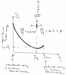
the equilibrium value of $\xi$ corresponds with $\Delta_r G=0$ . Furthermore, if the reactive mixture happens to have been prepared away from the equilibrium composition, the direction of the process will be determined by the sign of $\Delta_r G$ , since for $\xi < \xi_\text{eq}$ , $\Delta_r G< 0$ , and so $\xi$ will be increasing until it reaches its equilibrium value and vice versa for $\xi > \xi_\text{eq}$ . We summarize these notions in the Table below:

$\Delta_r G < 0$

$d \xi > 0$

reaction will proceed as written

$\Delta_r G > 0$

$d \xi < 0$

reaction will proceed in the opposite direction

$\Delta_r G = 0$

$d \xi = 0$

the reactive mixture is already at equilibrium

It is straightforward to obtain an explicit expression for the Gibbs free energy of a gas reaction in the approximation of the gases being nearly ideal. We will use the expression for the chemical potential we had obtained in Chapter 7, which we re-write here per mole:

(16) $\begin{equation*} \mu \:=\: - R T \ln \left[ \left( \frac{T}{e T^\ominus} \right)^{c_V/k_B} \left( \frac{V}{V^\ominus} \right) \right] \end{equation*}$

To make it a function exclusively of temperature and pressure, we will use the ideal gas law $pV=N k_B T$ and standard formulas $x \ln y = \ln y^x$ and $\ln x + \ln y = \ln (xy)$ to obtain $\mu = RT \ln(p \, T^{-c_V/k_B-1} \times \text{const})$ , where the constant depends on the standard pressure and temperature and, also, contains numerical factors. In much of the following, we will set the temperature to its standard value, which, then, yields a greatly simplified expression for the chemical potential:

(17) $\begin{equation*} \mu \:=\: \mu^\ominus \:+\: RT \ln(p/p^\ominus) \end{equation*}$

Note that this expression can be used to evaluate the chemical potential of the gas when the gas is part of a gas mixture but $p$ now stands for the partial pressure of the gas in the mixture. Indeed, Eq. 16 contains the full volume of the system, and so the equation of state $p_i =N_i k_B T/V$ , where $N_i$ is the particle number for component $i$ , gives the pressure due to the component $i$ exclusively, irrespective of whether other components are present or not.

Now consider, for the sake of argument, the very simplest reaction

A = B

and assign species B to be the product and species A the reactant:

B – A = 0

Thus

$\nu$ _A = $1-\xi$

and

$\nu$ _B = $\xi$

Assume further that this is a gas reaction and that the gases are nearly ideal. If the total pressure is $p$ , the partial pressures of the species A and B, respectively, are given by:

(18) $\begin{equation*} p_A = \frac{\nu_A}{\nu_A+\nu_B}\: p = (1-\xi) \: p \end{equation*}$

and

(19) $\begin{equation*} p_B = \frac{\nu_B}{\nu_A+\nu_B} \: p = \xi \: p \end{equation*}$

because $p_A=N_A k_B T/V$ and $p_B=N_B k_B T/V$ , while $p=(N_A+N_B) k_B T/V$ . Note that the chemical potentials of both species A and B depend on the mole fractions of the components, as was alluded to earlier.

Substituting the partial pressures in the respective expressions for the chemical potentials in Eq. 10, one obtains the following expression for the overall (non-equilibrium) Gibbs energy:

(20) $\begin{eqnarray*} \tilde{G} &=& n_A \mu_A \:+\: n_B \mu_B \\ &=& (1-\xi) [\mu_A^\ominus \:+\:RT \ln(p_A/p^\ominus) ] \:+\: \xi [\mu_B^\ominus \:+\:RT \ln(p_B/p^\ominus ] \end{eqnarray*}$

thus leading to

(21) $\begin{equation*} \tilde{G} \: = \: \mu_A^\ominus + \xi (\mu_B^\ominus - \mu_A^\ominus) \:+\:RT \ln(p/p^\ominus) \:+\: RT [ \xi \ln \xi + (1-\xi) \ln (1-\xi) ] \end{equation*}$

In this expression, we recognize the last term as that arising from the entropy of mixing: $-TS_\text{mix}$ . One can easily check that the remaining terms are a weighted sum of the chemical potentials of pure species A and B, respectively, the weights determined the corresponding mole fractions.

The mixing contribution has an important mathematical property that its derivatives are infinite at the l.h.s. and r.h.s. edges of interval of allowed values of $\xi$ . At the same time, the slope of the remaining $\xi$ dependence is finite throughout. This implies that the minimum of the non-equilibrium Gibbs energy is necessarily contained within the interval.

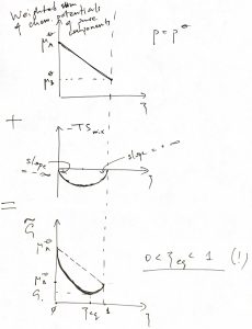
This means that the reaction always proceeds at least to some extent but, at the same time, never proceeds to full completion! This interesting entropic effect comes about, physically, because no matter how unfavorable the reactants or products might be, once formed they will have the whole volume of the system at their disposal. For this very reason, it is very hard to purify a substance or, for instance, fully eliminate crime in a large city. On the good side, it also means that a large city is essentially guranteed to have exceptionally good people, too!

By analogy with the expression for the chemical potential of an ideal gas of species $i$

(22) $\begin{equation*} \mu_i \:=\: \mu_i^\ominus \:+\: RT \ln(p_i/p^\ominus) \end{equation*}$

be the species in pure form or a part of a gaseous mixture, we use the following formal expression for the chemical potential of species $i$ in any physical form:

(23) $\begin{equation*} \mu \:=\: \mu_i^\ominus \:+\: RT \ln a_i \end{equation*}$

where the quantity $a_i$ is called the activity. To reiterate,

(24) $\begin{equation*} a_i = p_i/p^\ominus \text{ for ideal gases} \end{equation*}$

For non-ideal gases, on the other hand, $a_i = \gamma_i p/p^\ominus$ , where $\gamma$ is called the fugacity coefficient (the combination $\gamma p$ is called the fugacity) and $p$ is the total pressure. Note that for non-ideal gases, one can no longer define partial pressures since distinct components now interact. For liquid mixtures, we take the respective pure substances as the standard states, and so, by definition, $a_i=1$ in the standard state. The rationale behind the convention 23 is not solely formal: In the limit of low mole fraction of the species $i$ one can think of it as a dilute “gas” of molecules of this species while the rest of the liquid mixture can be thought of as an effective vacuum that can be described effectively as a vacuum but with somewhat distinct properties from the actual vacuum. Since the molecules of this effective “gas” do not interact with each other, we expect the activity to scale linearly with its concentration

(25) $\begin{equation*} a_i \propto [i], \text{ at low values of concentration }[i] \end{equation*}$

as if the species were a nearly ideal gas.

It is instructive to express the reaction’s Gibbs energy through the activities:

(26) $\begin{eqnarray*} \Delta_r G &\equiv& \sum_{i=1}^{M} \nu_i \mu_i \\ & \equiv & \sum_{i=1}^{M} \nu_i (\mu_i^\ominus \:+\: RT \ln a_i) \\ &=& \sum_{i=1}^{M} \nu_i \mu_i^\ominus \:+\: RT \sum_{i=1}^{M} \nu_i \ln a_i \\ & = & \Delta_r G^\ominus \:+\: RT \ln \prod_{i=1}^{M} a_i^{\nu_i} \\ & = & \Delta_r G^\ominus \:+\: RT \ln Q \end{eqnarray*}$

where we have defined the standard Gibbs energy of the reaction

(27) $\begin{equation*} \Delta_r G^\ominus \equiv \sum_{i=1}^{M} \nu_i \mu_i^\ominus \end{equation*}$

and the so called reaction quotient

(28) $\begin{equation*} Q \equiv \prod_{i=1}^{M} a_i^{\nu_i} \end{equation*}$

The reaction quotient looks like a rather formal object yet it is the only systematic way to quantify the balance between the reactants and products. For instance, consider the dilute limit of the gas reaction 2H₂O – 2H₂ – O₂= 0. Hereby, the activity of each component is proportional to its concentration, and so $Q \propto \frac{[\text{H}_2 \text{O}]^2}{[\text{H}_2]^2 [\text{O}_2]}$ , which makes perfect sense: The chances of the reaction proceeding in the direction as written is determined by the probability of bringing together two hydrogen molecules and one oxygen molecule, which is proportional to the product $[\text{H}_2] [\text{H}_2] [\text{O}_2]=[\text{H}_2]^2 [\text{O}_2]$ . (Recall that the probabilities of independent events multiply and that the probability to find a molecule is proportional to the concentration of that molecule.) On the other hand, since the reaction produces two water molecules, the probability of the reverse process is determined by the chances of bringing together two water molecules. Thus the proper measure of the probability to be in the “product state” of the system relative to the “reactant state of the system” is given by the reaction quotient.

What is the equilibrium value of the reaction quotient? According to the Table above, the reactive mixture is in equilibrium, if $\Delta G_r = 0$ . Thus, by Eq. 26, we have at equilibrium

(29) $\begin{equation*} \Delta_r G^\ominus \:+\: RT \ln Q_\text{eq} \:=\: 0 \end{equation*}$

The equilibrium value of the reaction constant is rather special and has its own name: the equilibrium constant:

(30) $\begin{equation*} K \: \equiv \: Q_\text{eq} \end{equation*}$

Thus we obtain that the equilibrium constant, i.e., the equilibrium value of the reaction quotient has the following relation with with the standard Gibbs free energy:

(31) $\begin{equation*} K \: = \: e^{-\Delta_r G^\ominus/RT} \end{equation*}$

Not surprisingly, we obtain that the probability of being in the product relative to reactant state is given by the relative Boltzmann weight of the two states, in complete consonance with our developments so far.

Note that to each value of temperature there corresponds a unique value of the equilibrium constant. Moreover, the equilibrium constant is exclusively a function of temperature, but not pressure since the standard pressure is fixed, by convention.

The above notions can be used to analyze the pressure dependence of the chemical equilibrium. As an example, consider the following simple gas reaction, where a weak complex N₂O₄ (reversibly) falls apart into two identical molecules NO₂:

N₂O₄ = 2 NO₂

According to Eq. 12, $n_{\text{NO}_2}=2 \, \xi$ , and $n_{\text{N}_2 \text{O}_4}=1-\xi$ while the total amount is $2\xi + (1-\xi)=1+\xi$ . Thus:

N₂O₄

NO₂

initial amount

1

0

equilibrium amount

$1-\xi_\text{eq}$

$2 \, \xi_\text{eq}$

equilibrium mole fraction

$\frac{1-\xi_\text{eq}}{1+\xi_\text{eq}}$

$\frac{2 \, \xi_\text{eq}}{1+\xi_\text{eq}}$

partial pressure in equilibrium

$p_{\text{NO}_2}=\frac{1-\xi_\text{eq}}{1+\xi_\text{eq}} \, p$

$p_{\text{N}_2\text{O}_4} = \frac{2 \, \xi_\text{eq}}{1+\xi_\text{eq}} \, p$

where $p$ is the total pressure: $p=p_{\text{NO}_2}+p_{\text{N}_2\text{O}_4}$ . This yields for the equilibrium constant, after simple algebra:

(32) $\begin{eqnarray*} K &=& \frac{(p_{\text{NO}_2}/p^\ominus)^2}{p_{\text{N}_2 \text{O}_4}/p^\ominus} \\ &=& \frac{\xi_\text{eq}^2}{1-\xi_\text{eq}^2} \: \frac{p}{p^\ominus} \end{eqnarray*}$

The relation between the equilibrium constant and the equilibrium value of the reaction coordinate we just obtained happens to be simple enough that we can solve it for $\xi_\text{eq}$ in terms of pressure and the equilibrium constant:

(33) $\begin{equation*} \xi_\text{eq}\:=\:\frac{1}{[1\:+\:\frac{4}{K} \: \frac{p}{p^\ominus}]^{1/2}} \end{equation*}$

We plot it here as a function of pressure for three select values of $K$ :

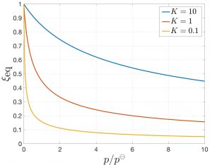
Clearly, the amount of products decreases with pressure. This is expected since the volume of the product is greater than the volume of the reactants, per mass. Thus one can shift the equilibrium toward reactants by increasing the pressure and toward products by reducing the pressure. This is an example of the Le Chatelier principle, whereby the system responds so as to compensate the external influence. Indeed, by reducing the volume of the mixture, the system “mitigates” our attempt to increase its pressure. We also see the amount of products increases with the equilibrium constant, as expected.

In addition to the direction of a chemical process, of interest is also the heat, or, enthalpy of the reaction since it determines how much heat will be produced or consumed during the reaction. In the former case, one must be able to sequester the heat to avoid explosion while in the latter case, one must supply heat in order for the reaction to take place. Note that in either case, the kinetics are important because what matters is how much heat is produced/consumed in unit time. Here we are mostly concerned with the thermodynamics, i.e., the total amount of heat produced or consumed. This amount is determined by the amount of reactive mixture and the extent of deviation from equilibrium; it does not depend on the kinetics of the process.

To determine the enthalpy of the reaction we first derive a differential relation between $G$ and $H$ . For a pure substance,

(34) $\begin{equation*} H=G+TS=G-T\left(\frac{\partial G}{\partial T}\right)_{p, N}=\frac{\partial [(1/T) G]}{\partial (1/T)}= \frac{\partial (G/T)}{\partial (1/T)}\end{equation*}$

where we used that $d(1/T)/d(1/T)=1$ and $-T^2 (dG/dT)=\frac{dG}{-\frac{1}{T^2}dT}=dG/d(1/T)$ . We also assume that pressure and particle number remain constant.

The same relation holds for the enthalpy and Gibbs energy per mole, as can be seen by dividing out the above equation by number of moles:

(35) $\begin{equation*} h_i = \frac{\partial (\mu_i/T)}{\partial (1/T)}\end{equation*}$

where we have added the label $i$ to allow us to write this equation for different species and remembered that the chemical potential is the Gibbs energy per mole.

Let us define the reaction enthalpy analogously to the reaction Gibbs energy

(36) $\begin{equation*} \Delta_r H \:\equiv \: \sum_{i=1}^{M} \nu_i \, h_i \end{equation*}$

Multiplying the Eq. 35 by $\nu_i$ and summing over the species, $i=1 \ldots M$ , yields

(37) $\begin{equation*} \sum_i^M \nu_i h_i = \frac{\partial (\sum_i^M \nu_i \mu_i/T)}{\partial (1/T)}\end{equation*}$

thus yielding

(38) $\begin{equation*} \Delta_r H = \frac{\partial (\Delta_r G/T)}{\partial (1/T)}\end{equation*}$

where, again, the pressure and particle number for each species is held constant, and we used the definition of the reaction Gibbs energy 14. On the other hand, according to Eq. 31, the standard Gibbs energy

(39) $\begin{equation*} \Delta_r G^\ominus/T \:=\: -R \ln K \end{equation*}$

is a pressure independent quantity and does not depend on the particle number either. Thus we obtain that the standard reaction enthalpy obeys the following equation:

(40) $\begin{equation*} \Delta_r H^\ominus = -R \, \frac{d \ln K}{d (1/T)} \end{equation*}$

where we were able to replace the partial derivative w.r.t. $T$ with the full derivative since $T$ is the only variable. This equation—which is often referred to as the van’t Hoff equation— is particularly useful when the reaction enthalpy happens to be temperature independent or nearly so. Indeed, under these circumstances, the equation above implies the dependence of $\ln K$ on the inverse temperature is simply a straight line:

(41) $\begin{equation*} \ln K= -\frac{ \Delta_r H^\ominus}{R} \frac{1}{T} + \text{const} \end{equation*}$

We can fix the constant by defining the reaction’s entropy:

(42) $\begin{equation*} \Delta_r S \:\equiv \: \sum_{i=1}^{M} \nu_i \, s_i \end{equation*}$

( $s_i$ stands for the molar entropy of component $i$ ) and using the general formula that $G=H-TS$ , which, then, implies $\Delta_r G=\Delta_r H-T \Delta_r S$ . This and the usual $\ln K = -RT \Delta_r G^\ominus$ yield

(43) $\begin{equation*} \ln K= -\frac{ \Delta_r H^\ominus}{R} \frac{1}{T} + \frac{ \Delta_r S^\ominus}{R} \end{equation*}$

This mathematical statement, which was derived assuming $\Delta_r H$ is temperature independent, automatically implies that the standard reaction entropy is then temperature independent as well. The above equation is quite useful as it allows one to determine both the reaction’s enthalpy and entropy by plotting the equilibrium constant as a function of inverse temperature:

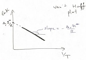
In the above picture, $\Delta_r H > 0$ , which formally implies that the reaction is endothermal, i.e., consumes heat. The resulting $T$ -dependence of the equilibrium constant is yet another instance of Le Chatelier’s principle: As one attempts to raise the temperature by putting in heat, the equilibrium shifts toward the higher enthalpy state (products in this case) so as to absorb that heat. The converse is also true: Raising the temperature of an exothermal process, $\Delta_r H < 0$ , will shift the equilibrium toward the reactants.

Note that in physical terms, $\Delta_r H > 0$ means that, on average, one must break bonds to create the product. On the other hand, heat production, $\Delta_r H < 0$ , means the bonds in the molecules comprising the products are stronger than the bonds in the molecules comprising the reactants. This notion underlies the heat production during burning or, more, generally, oxidation of fossil fuels, of course.

Before we attempt a chemical reaction, it is useful to estimate beforehand both the reaction’s Gibbs energy and enthalpy, as we have already indicated. Making such estimates from scratch is difficult. Approximate estimates are, however, still possible for a huge variety of distinct reactions since the enthalpies of pure components can be—and in many cases have been—measured. Ignoring, then, the affect of mixing of the individual components with each other, we can present the thermodynamic path from the reactant to the product state as one going through some standard state. And so, for instance, for a reaction:

$\nu$ _A A + $\nu$ _B B = $\nu$ _C C + $\nu$ _D D

this mental construction looks something like this:

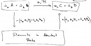
This is as if one decided to travel from city X (our reactants) to city Y (our products) not directly, but through some city Z (the standard state). Clearly, if one knows the elevation of city X relative to city Z, $h_X-h_Z$ , and the elevation of city Y relative to city Z, $h_Y-h_Z$ , one can compute the elevation of Y relative to X: $(h_Y-h_Z)-(h_X-h_Z)= h_Y-h_X$ . By exactly the same token, the enthalpy is a state function and so the enthalpy difference between two states depends on the identity of those states irrespective of the path one uses to go between the states. The enthalpy of the standard-state to the product-state process is given by $(\nu_C \Delta_f H_C\:+\:\nu_D \Delta_f H_D)$ , where we used the subscript $f$ to signify “formation”. Likewise, the enthalpy of the standard-state to the reactant-state process is given by $(\nu_A \Delta_f H_A\:+\:\nu_B \Delta_f H_B)$ . Therefore the enthalpy of the reactant→product process is equal to the enthalpy of the reactant→standard-state→product process:

(44) $\begin{equation*} \Delta_r H \:=\:(\nu_C \Delta_f H_C\:+\:\nu_D \Delta_f H_D)\:-\:(\nu_A \Delta_f H_A\:+\:\nu_B\Delta_f H_B) \end{equation*}$

where the minus sign reflects that the reactant→standard-state leg is in the opposite direction of actually bringing the constituent elements from the standard state to the reactants state. Note that the formation enthalpies $\Delta_f H$ are usually given per mole. This is distinct from the convention adopted in this Course whereby we have attempted to consistently denote quantities per particle or per mole using low-case letters.

Because the Gibbs energy and the entropy are state functions, one can write down equations for the reaction’s Gibbs energy and the reaction’s entropy that are entirely analogous to the equation above.

Actual estimates the formation entropy and enthalpy depend on the convention for the standard state. As an example, consider the following procedure: We can use the 3rd Law of Thermodynamics, $S(T=0)=0$ , to define our reference state. Given this, the entropy at any temperature can be computed by integrating the equation for the heat capacity $C_p = T(\partial S/\partial T)_p$ so long as there is no discontinuous transition takes place:

(45) $\begin{equation*} S(T) = S(T=0) + \int_0^T \frac{c_p}{T} dT = \int_0^T \frac{c_p}{T} dT \end{equation*}$

And, likewise for the enthalpy, where one can inegrate the relation $C_p=(\partial H/\partial T)_p$ :

(46) $\begin{equation*} H(T) - H(T=0)= \int_0^T \, c_p dT \end{equation*}$

If there is, in fact, a phase transition at some temperature, one must add a constant value equal to the transition’s entropy at that temperature. Thus the $T$ -dependence of the entropy will look something like this:

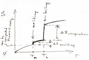
The $T$ -dependence of the enthalpy is qualitatively similar. Consequently, one can compute the Gibbs energy $G=H-TS$ , which, recall, is a continuous function of temperature. In practice, it is often most straightforward to actually compute the heat capacity of solids, while the heat capacity in the liquid and vapor state is often easier to measure, as are the heats of melting and boiling.

The fact of the enthalpy being a state function allows one to straightforwardly to evaluate the enthalpy at condition other than those readily accessible in the lab. For instance the enthalpy of the reaction

2H (gas) = H₂ (gas)

at $T=0$ K can be estimated using the measured enthalpy of the reaction at a more accessible temperature using the following construction:

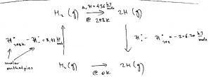
One, then, finds straightforwardly

(47) $\begin{equation*} \Delta_r H\:(T=0 \text{K})\:=\:(8.47\:+\:436\:-\:12.4)\:\text{kJ/mole}\:=\:432\:\text{kJ/mole}\end{equation*}$

The $T=0$ K estimate is not as arcane as one may seem because it can be directly compared with the output of quantum-chemical calculation, which produce most accurate results for the ground state of the system.

The above example is also revealing in the following sense: It illustrates just how much more enthalpy is “stored” in a chemical bond compared with a physical process such as heating or cooling. The enthalpy of the latter processes is clearly comparable to the thermal energy $RT$ , which, then, brings about another important point. The thermal energy scale $RT$ , in gases, is also comparable to the quantity $p V_m$ , where $V_m$ is the molar volume. On the other hand, the energy and enthalpy are related through the equation $H=E+pV$ . Thus we conclude that the energy and enthalpy of a chemical bond are numerically close. This should have been expected: Bonding energies are of order several eV, while the thermal scale, $k_B T$ , at room temperature is about 1/40 eV. These are useful notions since quantum-chemical calculations actually produce the energy of the bond, while the experiment produces the bond’s enthalpy. Thus equating the two is, generally, an approximation, albeit a good one.

As another illustration of how one can exploit the fact of the enthalpy being a state function, we can determine the enthalpy of the H-O bond, per bond, in a water molecule:

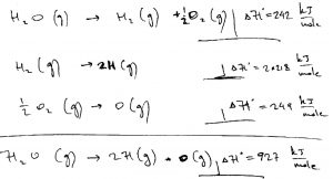
Note the actual strength of the H-OH bond and the H-O bond are not the same, the latter being significantly stronger than the former.

Our final remarks concern the kinetics of chemical processes. The thermodynamic considerations above do not directly address the issue of how fast the chemical processes in question will actually occur. This should have been clear already because nowhere in the discussion have we even mentioned the mass of the species. But we know that the mass is of decisive importance for how fast molecules move about, given that the typical energy scale for their motion is fixed by the temperature. What thermodynamics can do is tell us about the relative rates of processes in equilibrium. And so, for instance, we have written the relation between the equilibrium constant and the reaction’s Gibbs energy:

(48) $\begin{equation*} K \: = \: e^{-\Delta_r G^\ominus/RT} \end{equation*}$

As already mentioned, the equilibrium constant should be thought of as the probability of being in the product state relative to the probability of being in the reactant state. On the other hand, this probability must be equal to the ratio of the rates $\frac{k_{\text{reactants}\to \text{products}}}{k_{\text{products}\to \text{reactants}}}$ . Indeed, the probability of being in a state is proportional to the flux of the particles toward that state. Thus we obtain an example of what one calls the detailed balance:

(49) $\begin{equation*} \frac{k_{\text{reactants}\to \text{products}}}{k_{\text{products}\to \text{reactants}}} \: = \: e^{-\Delta_r G^\ominus/RT} \end{equation*}$

which essentially states that in equilibrium, the ratio of the transition rates between two states must match the free energy difference between the two states. We have already encountered a simpler version of the above statement, i.e., that the rates of transfer between two microstates 1 and 2 must obey the following relation:

(50) $\begin{equation*} \frac{k_{1 \to 2}}{k_{2 \to 1}} \: = \: e^{-(E_2-E_1)/k_B T} \end{equation*}$

Again, these relations do not tell us anything about the absolute values of the rate constants, only their ratios. The absolute values of rates contain time units. In order to obtain a quantity of units time from a quantity of units energy, one must use a quantity of units mass. The actual way to do this depends on the amount of quantum effects, to which we turn next.

License

Icon for the Creative Commons Attribution-NonCommercial-NoDerivatives 4.0 International License

Basic Notions of Thermodynamics and Quantum Mechanics for Natural Sciences Copyright © 2020 by Vassiliy Lubchenko is licensed under a Creative Commons Attribution-NonCommercial-NoDerivatives 4.0 International License, except where otherwise noted.

License

Share This Book