The Gibbs-Boltzmann distribution. The Maxwell distribution of velocities.

Vassiliy Lubchenko

5 The Gibbs-Boltzmann distribution. The Maxwell distribution of velocities.

In the preceding Chapter, we connected a dynamical description of matter at the molecular level with macroscopic observables, such as pressure and temperature, no small feat. Furthermore, we were able to make predictions about the time evolution of the system. To make the connection, we applied notions of statistics. We have assumed that there is a steady state ensemble of configurations (or “microstates”) the system will continue to revisit at a steady rate, on the average, and in no particular order. (The rate may be extremely small, but it should be non-vanishing. If a microstate has been visited once, it should be visited again and again in perpetuity.) The assumption of such recurrent sampling of all available configurations in random order—sometimes referred to as the “ergodic hypothesis”—is not innocent; its validity must be decided on a case to case basis. When the assumption does hold, one can say that the system can achieve equilibrium. Equilibrium is something that may take some time to establish after the system was prepared since there is no guarantee that the system was prepared in a typical configuration. This is analogous to the so called “beginners’ luck” in gambling, which typically runs out as the gambler continues to play. With these provisos in mind, let us now extend our treatment from nearly non-interacting gases to systems where particles actually interact; in the vast majority of systems of practical interest, interactions are present and are significant. We will continue to assume that equilibrium can be, in fact, established.

First off, what is “interaction”? In dynamical terms, interaction between two objects means that one object imposes some constraints on the motion of the other object. Consider the following energy function for two degrees of freedom:

(1) $\begin{eqnarray*} E &=& \frac{m_1 v^2_1}{2} + V_1(x_1) \\ &+& \frac{m_2 v^2_2}{2} + V_2(x_2) \\ &+& V_\text{int} (x_1, x_2) \end{eqnarray*}$

where $v_1 = dx_1/dt$ and $v_2 = dx_2/dt$ are the velocities corresponding to the degrees of freedom 1 and 2, respectively.

The top line on the r.h.s. contains terms that depend exclusively on the coordinate and velocity of particle 1. The middle line contains terms that depend exclusively on the coordinate and velocity of particle 2. In contrast, the bottom line contains a function that depends on the configuration of both particles. The full potential energy is, then, a sum of three terms:

(2) $\begin{equation*} V(x_1, x_2) = V_1(x_1) + V_2(x_2) + V_\text{int} (x_1, x_2) \end{equation*}$

By construction, the term $V_\text{int} (x_1, x_2)$ can not be decomposed into a sum of some function that depends solely on $x_1$ and some function that depends solely on $x_2$ :

(3) $\begin{equation*} V_\text{int} (x_1, x_2) \: \ne \: U(x_1) + U(x_2) \end{equation*}$

Clearly, then, the force acting on object 1 is modified by the presence of object 2, because differentiation with respect to $x_1$ does not rid us from the variable $x_2$ in the expression for the force acting on particle 1:

(4) $\begin{equation*} f_1 \:=\: -\frac{\partial V(x_1, x_2)}{\partial x_1} \:=\: -\frac{d V(x_1)}{d x_1}-\frac{\partial V_\text{int}(x_1, x_2) }{\partial x_1} \end{equation*}$

which is clearly a function of both $x_1$ and $x_2$ . Indeed, suppose, to the contrary, that $\frac{\partial V_\text{int}(x_1, x_2) }{\partial x_1}$ is not a function of $x_2$ , thus implying $\frac{\partial V_\text{int}(x_1, x_2) }{\partial x_1} = C_1(x_1)$ , where $C_1(x_1)$ is some function of $x_1$ but not $x_2$ . Integrating this equation with respect to $x_1$ yields $V_\text{int}(x_1, x_2) = \int^{x_1} C_1(x) dx + C_2$ , where $C_2$ is $x_1$ independent. ( $C_2$ could be a function of $x_2$ .) But this kind of additive form is expressly forbidden by the condition (3), thus proving that for non-additive potentials, object 2 exerts a force on object 1. By the same token, the force acting upon object 2 will depend on $x_1$ as well. The presence of a term $V_\text{int} (x_1, x_2)$ of the kind satisfying condition (3), in the full energy function, thus means the degrees of freedom in question are interacting, or “coupled”.

More generally, we can state that a set of degrees of freedom are non-interacting, if the full energy function is additive, i.e., it can be decomposed into a sum of energy functions each pertaining to an individual degree of freedom and there are no “cross-terms” that couple the degrees of freedom:

(5) $\begin{equation*} E \: = \: \sum_i E^{(i)} \Rightarrow \text{ no interaction} \end{equation*}$

where $E^{(i)} \equiv E^{(i)}(x_i, v_i)$ is the energy function for the degree of freedom $i$ .

The above notions on the additivity of energies of independent degrees of freedom have two very important implications:

Energy can be used as an indicator for whether interactions have actually occurred. Indeed, we saw that interactions change the state of the motion of the system—sometimes referred to as the “microstate”—since they amount to a non-vanishing force, by Eq. (4). Thus changes in the value of the energy can be used to bookkeep the microstates of a system. Indeed, two distinct values of energy necessarily correspond to two distinct microstates. The converse is not necessarily true, however. Furthermore, a great deal of ambiguity arises when two or more distinct microstates are degenerate, i.e, have the same value of energy. This ambiguity is thus intrinsically built into a bookkeeping scheme based on energies and, as we will see later, is impossible to avoid in practice. Fortunately, this complication can (and will) be dealt with and has colossal significance in applications.
The lack of mutual correlation between two degrees of freedom, whose energies simply add to make up the total energy, allows one to explicitly determine the functional form of the dependence of the probability $p_i$ of microstate $i$ on the energy $E_i$ of that microstate. This is because probabilities of independent events multiply, as we saw earlier.

Let’s work this out mathematically. Since we have agreed that the energy is the only quantity we will keep track of, the probability of microstate $i$ is determined exclusively by its energy $E_i$ :

(6) $\begin{equation*} p_i = \frac{g(E_i)}{Z} \end{equation*}$

where $g$ is a specific but unknown, as of yet, function, and the quantity

(7) $\begin{equation*} Z \equiv \sum_i g(E_i) \end{equation*}$

is a normalization factor ensuring our probabilities are normalized:

(8) $\begin{equation*} \sum_i p_i = \frac{1}{Z} \sum_i g(E_i) = \frac{1}{Z} \: Z = 1 \end{equation*}$

which formally reflects the notion that the system is in some microstate with probability one.

As written in Eq. (6), the definition of the function $g(E_i)$ is still ambiguous. Indeed, if we multiplied all of the $g(E_i)$ ‘s by a fixed number, the value of the weights $p_k$ would not change since $Z$ would also be multiplied by the same fixed number, by Eq. (7). To remove this ambiguity, we impose an additional condition that the quantity $Z$ be equal to the total number of accessible microstates, subject to some constraints of choice. (Common constraints include things like fixing the temperature and/or volume of the system, or maintaining a certain value of pressure and particle number, etc.) The (as of yet unknown function) $g(E_i)$ , then, can be thought of as the contribution of state $i$ to the total number of thermally available states. The number of accessible states has a spooky property that it does not have to be integer, in seeming conflict with the expectation that the number of configurations can obtained by ordering them in some way and then counting them using ordinal numbers. Likewise, the contribution $g(E_i)$ of state $i$ to the number of available states can be less than one! I will illustrate how this apparent lack of ordinality comes about using an example. Suppose you live in a 3-story home and your friend lives in a 5-story home; each story has exactly one room. Clearly you can be in one room at a time, and so there are 3 distinct configurations when you are home. Likewise, your friend has 5 distinct configurations, and the compound you+friend system has $3 \times 5 = 15$ distinct configurations. Indeed, for each of your 3 configurations, your friend has 5. Now suppose you really don’t like going upstairs much because your wi-fi router is on the ground floor and the signal quality deteriorates as your go upstairs. (This is your constraint.) As a result, you spend say, 60% of your time on floor 1, 30% on floor 2, and the remaining 10% on floor 3. Being the likeliest one, the 1st floor configuration is counted as unconditionally accessible and so contributes exactly 1 to the total number of accessible configurations. The 2nd floor configuration contributes only $\frac{30 \, \%}{60 \, \%}= \frac{1}{2}$ , and the 3rd floor configuration contributes only $\frac{10 \, \%}{60 \, \%}= \frac{1}{6}$ . The resulting accessible number of configurations is, then, $Z_1=1 + \frac{1}{2} + \frac{1}{6} = 1 \frac{7}{12} \approx 1.583$ . It is substantially less than the number of configurations that would be accessible without any constraints, i.e., 3. This type of reasoning may strike you as odd, so let’s look at a simpler yet more extreme example. Suppose you have a fair coin. Clearly there are exactly two distinct configurations: heads and tail. Correct? Now suppose the coin is slightly unfair, say, the odds of heads vs. tails are 5 vs. 4. How many accessible configurations does that correspond to? To drive home the point that this number is less than 2, imagine instead that the odds are grotesquely skewed toward heads, say, $e^{10^{23}}$ vs. $1$ . Nobody in their right mind would bet even a penny on the possibility of observing tails, since $1/e^{10^{23}}$ is equivalent to zero for all intents and purposes. This means that the accessible number of states for this grossly unfair coin is just one, the accessible state being the heads. The number of accessible states for the slightly unfair coin, in a sense, interpolates between the fair coin and the grossly unfair coin, yielding: $1+ \frac{4}{5} = 1.8$ . Now suppose your friend has a similar problem with her wi-fi in her house and her odds of being on floors 1 through 5 are, respectively: 40%, 30%, 20%, 7%, and 3%. The resulting number of accessible states is, then $Z_2= 1+\frac{30}{40} + \frac{20}{40} +\frac{7}{40} + \frac{3}{40} = 2.5 < 5$ . And what is the total number of accessible states for the compound you+friend system? It is $Z_1 \times Z_2 = 1\frac{7}{12} \times 2\frac{1}{2} \approx 3.96$ , well below the 15 states that would be accessible without the constraints.

Now consider a general compound system consisting of two non-interacting subsystems, 1 and 2, and label their microstates with indices $k_1$ and $k_2$ , respectively. The probability of microstate $k_1$ , whose energy is $E^{(1)}_{k_1}$ , is, then

(9) $\begin{equation*} p_{k_1}^{(1)} = \frac{1}{Z^{(1)}} g(E^{(1)}_{k_1}) \end{equation*}$

Likewise, the probability of microstate $k_2$ , whose energy is $E^{(2)}_{k_2}$ for system 2 is

(10) $\begin{equation*} p_{k_2}^{(2)} = \frac{1}{Z^{(2)}} g(E^{(2)}_{k_2}) \end{equation*}$

$Z^{(1)}$ is the number of accessible states for system 1 and $Z^{(2)}$ for system 2.

On the one hand, the probability to observe states $k_1$ and $k_2$ simultaneously is given by the product of the probabilities of the standalone probabilities, as we discussed in the preceding Chapter:

(11) $\begin{equation*} p_{k_1 k_2} \:=\: p_{k_1}^{(1)} \: p_{k_2}^{(2)} \end{equation*}$

One the other hand, Eq. (6) tells us the probability of the $(k_1, k_2)$ configuration is

(12) $\begin{equation*} p_{k_1 k_2} \:=\: \frac{1}{Z} \: g(E^{(1)}_{k_1}+E^{(2)}_{k_2}) \end{equation*}$

because the energy of the combined system is simply $E^{(1)}_{k_1}+E^{(2)}_{k_2}$ . Furthermore, the total number of accessible states is determined by multiplying those numbers for the standalone systems 1 and 2, as we discussed above:

(13) $\begin{equation*} Z \: = \: Z^{(1)} \: Z^{(2)} \end{equation*}$

Putting together Eqs. (28)-(13) yields

(14) $\begin{equation*} g(E^{(1)}_{k_1}+E^{(2)}_{k_2}) = g(E^{(1)}_{k_1}) \times g(E^{(2)}_{k_2}) \end{equation*}$

This equation applies for any values of the two quantities $E^{(1)}_{k_1}$ and $E^{(2)}_{k_2}$ and, thus, defines a functional equation for the (yet unknown) function $g(x)$ :

(15) $\begin{equation*} g(x+y) = g(x) \, g(y), \text{ for any two arguments } x \text{ and } y \end{equation*}$

Functional equations generally do not have a unique solution and are often hard to solve. But, in this particular case, we are in luck since the solution is not hard to find and is sufficiently unique for our purposes. First, set $y=0$ in Eq. (15) to convince yourself that

(16) $\begin{equation*} g(0) = 1 \end{equation*}$

Next, differentiate Eq. (15) with respect to $y$ , where one must use the chain rule for the l.h.s.: $\frac{\partial g(x+y)}{\partial y} = g'(x+y) \frac{\partial (x+y)}{\partial y} = g'(x+y) \times 1 = g'(x+y)$ , where the prime means the derivative with respect to the argument of the function:

(17) $\begin{equation*} f'(x) \:\equiv\: \frac{df}{dx} \end{equation*}$

And so one gets

(18) $\begin{equation*} g'(x+y) = g(x) \, g'(y) \end{equation*}$

Now again set $y=0$ to obtain

(19) $\begin{equation*} g'(x) \:=\: -\beta \: g(x) \end{equation*}$

where defined the constant $\beta$ to equal the negative derivative of $g$ at the origin:

(20) $\begin{equation*} \beta \:\equiv\: -g'(0) \:\equiv\: - dg/dx|_{x=0} \end{equation*}$

The minus sign is artificial but will make life easier in the future. Eq. (19) is easily solved by separating the variables and integrating: $dg/g \:=\: -\beta \, dx \: \Rightarrow \: \ln g \:=\: -\beta \, x + \text{const}$ , where the constant is fixed at $\text{const}=0$ , in view of Eq. (16). As a result, we obtain a remarkably simple expression for the function $g$ :

(21) $\begin{equation*} g(E) = e^{-\beta E} \end{equation*}$

We are left with determining the coefficient $\beta$ . Consider a particle freely moving in 1D (“moving freely” = “not subjected to an external force”): $E = \frac{m v_x^2}{2}$ , where I used the subscript $x$ to emphasize that the motion is along one spatial direction, chosen to be $x$ for concreteness. Distinct microstates of the particles differ only by their velocities and, in fact, are uniquely labelled by the corresponding value of $v_x$ itself. Hence,

(22) $\begin{equation*} p(v_x) \propto C e^{- \beta m v_x^2/2} \end{equation*}$

where the $v$ -independent proportionality constant can be determined by requiring that the distribution be normalized to 1: $\int_{-\infty}^{\infty} p(v_x) \, dv_x\:=\: 1$ . (The lack of dependence of the constant $C$ on the velocity is, perhaps, best appreciated in Quantum Mechanics, through the concept of “the phase space”, but see below, where we discuss the velocity distribution in 3D.) This yields, after consulting the table of definite integrals: $\int_{-\infty}^{\infty} e^{-\alpha y^2} dy \:=\: (\pi/\alpha)^{1/2}$ :

(23) $\begin{equation*} p(v_x) \: = \: \left(\frac{\beta m}{2 \pi} \right)^{1/2} e^{- \frac{\beta m v_x^2}{2}} \end{equation*}$

Next we compute the average of the velocity squared:

(24) $\begin{equation*} \langle v_x^2 \rangle \:\equiv\: \int_{-\infty}^{\infty} v_x^2 \: p(v_x) \, dv_x = \frac{1}{\beta m} \end{equation*}$

On the other hand, in the preceding Chapter we defined the temperature according to $k_B T = m \langle v_x^2 \rangle$ . This immediately yields:

(25) $\begin{equation*} \beta \: = \: \frac{1}{k_B T} \end{equation*}$

As a result we may write, for the probability of state $k$ , what is called the Gibbs-Boltzmann distribution:

(26) $\begin{equation*} p_i = \frac{e^{-\beta E_i} }{Z} \end{equation*}$

where the number of accessible states:

(27) $\begin{equation*} Z \equiv \sum_i e^{-\beta E_i} \end{equation*}$

is sometimes called the partition function, because it shows how the overall number of accessible states is partitioned among distinct microstates.

Eq. (26), together with Eqs. (25) and (27) of course, is arguably the most important result of Thermodynamics and Statistical Mechanics! The velocity distribution in Eq. (23) is also quite important in its own right. It is called the Maxwell distribution of velocities.

It is worthwhile to consider the simplest non-trivial arrangement where there two exactly two states. Such a two-level system is a good model for the electronic or nuclear spin 1/2 in a magnetic field. The two microstates correspond to the spin up and down. The lowest energy state is called the ground state. States at higher energies are called excited states. There is only one excited state in a two-level system, of course.

According to Eq. (6) and (7),

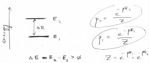
(28) $\begin{equation*} p_1 \:=\: \frac{e^{-\beta E_1}}{e^{-\beta\:E_1}\:+\:e^{-\beta E_2}}\:=\:\frac{1}{1\:+\:e^{-\beta \, \Delta E}}\end{equation*}$

and

(29) $\begin{equation*} p_2\:=\: \frac{e^{-\beta\, \Delta E }}{1\:+\:e^{-\beta\, \Delta E}}\end{equation*}$

Note $p_2\:=\:1\:-\:p_1$ , as it should, and that the probabilities depend only on energy differences, not the absolute values of energies. This is consistent with our earlier realization that only increments of the potential energy matter, not its absolute value. In other words, observable quantities should be independent of the energy reference. (Note forces are observable, energy is not!)

We next sketch the two weights $p_1$ and $p_2$ .

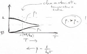
We note that $p_1 > p_2$ always, i.e., the ground state of the two-level system is always likelier to be occupied than the excited state. Only in the limit of infinite temperature, $T \to \infty$ , $\beta \to 0$ , do the two states become equally likely. Incidentally, this is the limit where the number of accessible states, $Z$ , approaches its largest possible value of 2.

Let’s review the meaning of the word “probability” in a practical context. One way to connect the weights $p_k$ to experiment is that given a (large) number $N$ of identical systems, we expect that at any given time: $N_1 = p_1 N$ will be in state 1, while $N_2 = p_2 N$ will be in state 2. Hereby,

(30) $\begin{equation*} p_1\:=\: \frac{N_1}{N_1+N_2} \end{equation*}$

(31) $\begin{equation*} p_2\:=\: \frac{N_2}{N_1+N_2} \:=\: 1 - p_1 \end{equation*}$

,

consistent with Eqs. (28) and (29). This is an example of ensemble averaging. Here you are looking at many equivalent systems at the same time.

Alternatively, one can determine the odds for a two-level system to be in state 1 or 2 by bookkeeping the amount time just one such system spent in those states. Here you monitor one system over a long time, this is called time averaging:

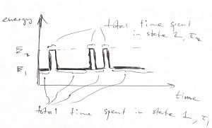
$p_1\:=\:\frac{\tau_1}{\tau_1\:+\: \tau_2}$

$p_2\:=\:\frac{\tau_2}{\tau_1\:+\:\tau_2}\:=\:1\:-\:p_1$

c.f. Eqs. (30) and (31).

Various quantities of interest can be determined using the statistical weights $p_1$ . For instance, the expectation (or average, or mean) value of the energy is

(32) $\begin{equation*} \langle E \rangle \:=\: \sum_i p_i \: E_i \:=\:E_1 p_1\:+\:E_2 p_2 \end{equation*}$

Note the expectation value of energy is never equal to its instantaneous value—i.e. the energy of either microstate—but, instead, interpolates between $E_1$ and $E)_2$ . Note also that because $p_2 < p_1$ , the largest energy the system can have is $\frac{E_1+E_2}{2}$ .

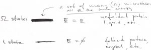
The only way to raise the expectation value of the energy is to employ more excited states. Consider, then, a more complicated example, where there is still just one ground state, at energy $E=0$ , but there are $\Omega$ excited states, each at energy $E= \varepsilon$ . The quantity $\Omega$ is often referred to as the degeneracy of the excited state. One must be careful and remembering that there are actually $\Omega$ distinct excited states.

As before, the probability to be in a particular state is determined by the Boltzmann-Gibbs distribution

(33) $\begin{equation*} p_i\:=\: \frac{e^{-\beta E_i}}{Z} \end{equation*}$

while the partition function $Z$ is given by

(34) $\begin{equation*} Z \:=\: \sum_i e^{-\beta E_i} = 1 + \Omega e^{-\beta \, \varepsilon} \end{equation*}$

We number the states starting from the ground state and use that $E_1 = 0$ and $E_i = \varepsilon$ for $i > 1$ , by construction.

The expectation value of the energy is now:

(35) $\begin{equation*} \langle E \rangle \:=\: \sum_i p_i \: E_i \:=\: \frac{ 1 }{ 1+\Omega\:e^{-\beta\varepsilon}} \:\: 0 \:+\: \frac{\Omega \: e^{-\beta \, \varepsilon} }{ 1+\Omega\:e^{-\beta\varepsilon}} \:\: \varepsilon \end{equation*}$

where we wrote out explicitly the ground and excited state energies $0$ and $\varepsilon$ to drive home that the question of the probability to have a certain amount of energy is generally very different from the question of the probability to be in a microstate with that energy.

Indeed, the probability to have energy $E = \varepsilon$ is

(36) $\begin{equation*} p(E=\varepsilon}) \:=\: \sum_{i: \: E_i = \varepsilon} p_i \:=\: \frac{\Omega \: e^{-\beta \, \varepsilon} }{ 1+\Omega\:e^{-\beta\varepsilon}}\end{equation*}$

and can be made as close to one as we want by making the degeneracy $\Omega$ larger.

It may be simple, but this model is not a bad approximation for the energy landscape of a protein molecule. Here the ground, lowest energy state would correspond to the protein molecule folded in its native state. Each of the unfolded states is significantly higher in energy than the native state and, individually, have no chance against the native state. When considered together, however, the unfolded states can take over given a high enough temperature. Indeed the probability to be unfolded relative to being folded is given by ratio:

(37) $\begin{equation*} \frac{p(E=\varepsilon)}{p(E=0)} \:=\: \Omega \: e^{-\beta \, \varepsilon} \end{equation*}$

At the special value of temperature, called the folding temperature $T_f$ , this ratio is equal to one implying the protein molecule is equally likely to folded or unfolded. Thus,

(38) $\begin{equation*} k_B T_f = \frac{\varepsilon}{ \ln \Omega} \end{equation*}$

Can you see that at $T> T_f$ , the $\frac{p(E=\varepsilon)}{p(E=0})}$ is greater than one, implying the protein molecule is likely unfolded? And vice versa for $T < T_f$ . Your homework problems highlight just how readily the equilibrium is shifted toward the folded state or the unfolded states as the temperature is moved away from $T_f$ . In any event, increasing the multiplicity of the unfolded states clearly decreases the folding temperature. This makes sense, doesn’t it?

It is now time for another Digression on Statistics: We saw just moments ago that in some cases, a variable that one can use to label distinct microstates is a truly continuous variable, such as the velocity in Eq. (23). This does not prevent one from histogramming this variable, of course, but it may now be practical to use a histogram where the width of the bar is arbitrarily narrow. One reason to do this is that if in the limit of a vanishingly narrow histogram bin, the histogram becomes smooth and, hence, becomes amenable to a variety of mathematical operations, such as differentiation. Integration becomes much easier, too. One problem with shrinking the bin size is that the number of data points decreases, too, roughly proportionally with the bin size. Indeed, now there are fewer data points per bin. Below I show two sets of the weights $p_k$ for the same data set. The two probability distributions correspond to two different values of the bin width:

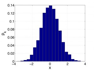
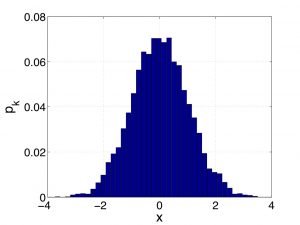
Clearly, in the limit of the vanishing bin size, the weights will vanish, too, at the same rate as the bin size does. To handle this, let us remind ourselves the definition of the average of some function $f(x)$ over a set of data points:

(39) $\begin{equation*} \langle f(x) \rangle\:\equiv\:\frac{1}{N}\sum_{i}^{N} f(x_i) \end{equation*}$

When the number $N$ of data is large, we may benefit from grouping the data into $M \ll N$ bins, just like we did it Chapter 2:

(40) $\begin{equation*} \langle f(x) \rangle\:\equiv\:\frac{1}{N}\sum_{i}^{N} f(x_i) \:=\:\sum_{k}^{M} \frac{N_k}{N} \tilde{f}(x_k) \:\equiv\:\sum_{k}^{M} p_k \tilde{f}(x_k) \end{equation*}$

where the index $k$ labels bins and $\tilde{f}(x_k)$ is the value of $f(x)$ averaged over bin $k$ . The weight $p_k \equiv N_k/N$ thus gives the partial quantity of the data falling within bin $k$ , as before.

(41) $\begin{equation*} \langle f(x) \rangle\:=\:\sum_{k}^{M} \Delta x_k \frac{p_k}{\Delta x_k} \tilde{f}(x_k) \end{equation*}$

where where $\Delta x_k$ is the width of bin $k$ . Since the weight $p_k$ scales linearly with $\Delta x_k$ , the ratio $p_k/\Delta x_k$ remains finite in the $\Delta x_k \to 0$ limit and we are justified in defining the following function:

(42) $\begin{equation*} p(x) \:\equiv\: \lim_{\Delta x_k \to 0} \frac{p_k}{\Delta x_k} \end{equation*}$

called the probability density. It is the continuous analog of the discrete distribution function $p_k$ . With this definition, the average in Eq. (43) can be rewritten as a definite integral:

(43) $\begin{equation*} \langle f(x) \rangle\:=\: \lim_{\Delta x_k \to 0} \sum_{k}^{M} \Delta x_k \: \frac{p_k}{\Delta x_k} \: \tilde{f}(x_k) \:=\: \int_{x_\text{min}}^{x_\text{max}} dx \: p(x) \: f(x) \end{equation*}$

,

where $x_\text{min}$ and $x_\text{max}$ delineate the range of the variable $x$ . According to its definition (42), the function $p(x)=\frac{N_k}{\Delta x_k} \, N$ is the number of points per unit interval, times the total number of data $N$ . Accordingly, the quantity $p(x)$ has dimensions of inverse $x$ . In this sense, it is a probability density. Accordingly, when we average over the distribution, we integrate, not sum. Note that the probability density $p(x)$ is normalized to one, if the parent distribution $p_k$ is:

(44) $\begin{equation*} \int_{x_\text{min}}^{x_\text{max}} dx \: p(x) \:=\: \lim_{\Delta x_k \to 0} \sum_{k}^{M} \Delta x_k \: \frac{p_k}{\Delta x_k} \:=\: \sum_k p_k \:=\: 1 \end{equation*}$

One may say that the quantity $p(x) \, dx$ gives the partial quantity of data falling within the (infinitesimal) interval $dx$ centered at $x$ . One may also say that the function $p(x)$ is the inverse of the typical spacing between the data points $\Delta x_k/N_k$ , times the total number of data $N$ .

Because the quantity $p(x) \, dx$ vanishes for an infinitely narrow interval $dx$ , one may say that the probability to for the variable $x$ to have a precise value, say $x_0$ , is strictly zero. However, it is better to remember that the question of the probability to have a specific value is not well posed. When we have continuous distributions, we, instead ask questions like this: What is the probability for the variable $x$ to be contained with an interval, say, $[x_1, x_2]$ . This kind of question is answered by computing an integral:

(45) $\begin{equation*} p(x_1 \le x \le x_2) = \int_{x_1}^{x_2} \, p(x) \, dx \end{equation*}$

which could be thought of as counting all of the data within the $[x_1, x_2]$ of a histogram. As an example of using Eq. (45), consider finding the median $x_m$ of a distribution. It is simply the value of the variable that splits the distribution exactly in two equal parts:

(46) $\begin{equation*} \int_{x_\text{min}}^{x_m} \, p(x) \, dx \:=\: \int^{x_\text{max}}_{x_m} \, p(x) \, dx \:=\: \frac{1}{2} \end{equation*}$

the last equation valid for distributions that are normalized to one. Although the median and the average of a distribution often follow each other, the median is sometimes preferable to the average, especially when the average does not even exist ( $\int \, x \: p(x) \: dx = \infty$ ). The latter situations will not be encountered in this Course, but they do arise when the distribution in question has very long tails, i.e., the probability density decays to zero slowly. (It must to decay to zero eventually, or, else, it would not be normalizable.) Working with the median is often more convenient also when, for instance, the distribution is bimodal so that the values of the variable that are numerically close to the average of the distribution are not particularly representative of the distribution.

Similarly to the probability distribution for a single physical quantity, we can define a distribution density for more than one distributed variable at at time. For instance, one can define a two-variable probability density according to

(47) $\begin{equation*} p(x, y) \:\equiv\: \lim_{\Delta x_{k_1}, \Delta y_{k_2} \to 0} \:\:\: \frac{p_{k_1 k_2}}{\Delta x_{k_1} \, \Delta y_{k_2} } \end{equation*}$

One can then compute the average of any function of $x$ and $y$ by evaluating a double integral:

(48) $\begin{equation*} \langle f(x, y) \rangle\:=\: \iint dx \, dy \: p(x, y) \: f(x, y) \end{equation*}$

where we did not write out the integration limits for typographical clarity. When both the averaged function and the distribution factorize, the above integration reduces to a product of two 1D integrals:

(49) $\begin{eqnarray*} \langle f_1(x) f_2(y) \rangle\:&=&\: \iint dx \, dy \: \: p_1(x) p_2(y) \:\: f_1(x) \, f_2(y) \\ \:&=&\: \left[ \int dx \: p_1(x) \: f_1(x) \right] \times \left[ \int dy \: p_2(y) \: f_2(y) \right] \end{eqnarray*}$

End of digression on Statistics.

The Gibbs-Boltzmann distribution is used to evaluate the probability of discretely distinct configurations (such as pregnant vs. not pregnant) and is not always straightforward to apply to situations where the variable labeling microscopic states seems to change continuously. This ambiguity is solved, more or less, in Quantum Mechanics. In the absence of a more rigorous treatment, we’ll try to get away with consistency-type reasoning. For instance, we can use the Gibbs-Boltzmann distribution to write down the probability distribution for the coordinate and velocity of a particle moving in 1D subject to the potential $V(x)$ :

(50) $\begin{equation*} p(v, x) \:=\: C \, e^{-\beta [mv_x^2/2 + V(x)]} \end{equation*}$

because the energy of the particle is $E = mv_x^2/2 + V(x)$ . We can reasonably guess that the constant $C$ in front of the exponential must be independent of $x$ . Indeed, shifting the potential over by length $x_0$ should simply shift the probability the distribution by the same length without multiplying it by some function of $x_0$ . The lack of dependence of $C$ on $v_x$ is a bit trickier. Here it helps to note that velocity changes, due to a non-vanishing force, do not explicitly depend on the velocity itself, according to Newton’s 2nd law: $m \Delta v = \int f \, dt$ , see also below. In any event, Eq. (51) encodes the remarkable fact that in equilibrium, the coordinate and velocity are statistically independent! Indeed the distribution (51) factorizes into an $x$ and $v$ dependent part:

(51) $\begin{equation*} p(v_x, x) \:=\: C \, e^{-\beta [mv_x^2/2 + V(x)]} \:=\: C \, e^{-\beta mv_x^2/2} \, e^{-\beta V(x)} \end{equation*}$

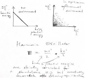
Consider, for instance, with the harmonic oscillator, whose kinetic and potential energies exactly anti-correlate in the absence of interaction with an environment. Once exposed to a thernal environment, the two energies will eventually decorrelated, the relaxation time depending on the efficiency of momentum transfer from the oscillator to the environment.

Now, the $x$ -dependent factor is sometimes called the Boltzmann distribution:

(52) $\begin{equation*} p(x) \:=\: A \, e^{-\beta V(x)} \end{equation*}$

where $A$ is a normalization constant that has no $x$ dependence.

An important example is the potential of the Earth’s gravity as as a function of height $z$ , relatively to the ground:

(53) $\begin{equation*} V(z) \,=\, m \, g \, z \end{equation*}$

It is easy to write down the resulting $z$ -dependence of the concentration of a gas because by its very meaning, the concentration of a gas at a specific location is proportional to the probability for a gas molecule to be at that location:

(54) $\begin{equation*} n(z) = n(z)|_{z=0} \: e^{-mgz/k_B T} \end{equation*}$

where $n(z)|_{z=0}$ is the concentration near the ground.

We sketch this $n(z)$ below:

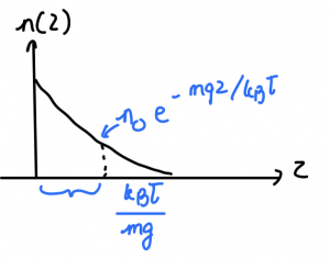
The exponential function decays very rapidly, the decay length in this particular case being determined by the quantity $k_B T/mg$ . Thus the thickness of the atmosphere is determined by the very same quantity $k_B T/mg$ . In reality, the temperature is not constant throughout the atmosphere and decreases quite rapidly with altitude, because of radiative cooling. As a result, the concentration profile will fall off with altitude even more rapidly as the isothermal, $T=\text{const}$ result would suggest. In any event, we arrive at a somewhat surprising result that the thickness of the atmosphere is determined not by the molecule’s size—consisent with the molecules not being in contact much of the time—but by how fast the molecules move!

We have already written down the velocity dependent part of the distribution (23) of velocities, i.e. the Maxwell distribution, for 1D motion. Its functional form is that of so called Gaussian distribution (named after the mathematician Gauss):

(55) $\begin{equation*} p(x) = \frac{1}{\sqrt{2 \pi \sigma^2}} e^{-\frac{(x-x_0)^2}{2 \sigma^2}} \end{equation*}$

with $x_0=0$ and $\sigma = (k_B T/m)^{1/2}$ . The distribution in Eq. (55) is also sometimes called the normal distribution and is incredibly important for this Course. You can convince yourself that the mean of the Gaussian distribution is given by

(56) $\begin{equation*} \langle x \rangle = x_0 \end{equation*}$

and variance

(57) $\begin{equation*} \langle (x - \langle x \rangle)^2 \rangle = \sigma^2 \end{equation*}$

The variance $\langle (x - \langle x \rangle)^2 \rangle$ is also sometimes called the mean square deviation (msd), while its square root:

(58) $\begin{equation*} \delta x \equiv \langle (x - \langle x \rangle)^2 \rangle^{1/2} \end{equation*}$

is called the root mean square deviation (rmsd), or the standard deviation. According to Eq. (57), the rmsd of the Gaussian distribution is numerically equal to the parameter $\sigma$ , a very simple result. As can be seen in the picture below, the rmsd is a good measure of the width of the Gaussian distribution:

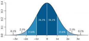
(By M. W. Toews. Own work, based (in concept) on figure by Jeremy Kemp, on 2005-02-09, CC BY 2.5, Link)

Indeed, we see that the $[-\sigma, \sigma]$ interval centered at the maximum $x_0$ of the distribution contains 68.2%, or so, of the data. A formal way to express this notion is: $\int_{x_0-\sigma}^{x_0+\sigma} p(x) \, dx \approx 0.682$ .

Now, we note that the mean velocity in all directions is zero:

(59) $\begin{equation*} \langle v_x \rangle = \langle v_y \rangle = \langle v_z \rangle = 0\end{equation*}$

This was obvious beforehand since the gas, as a whole, is not moving anywhere.

We are now ready to write the velocity distribution for motion in 3D. Because the contributions of the translations in the three spatial directions to the total energy are additive:

(60) $\begin{equation*} \frac{m \langle v ^2 \rangle}{2} \:=\: \frac{m\langle v_x^2 \rangle}{2}\:+\:\frac{m \langle v_y ^2 \rangle}{2}\:+\:\frac{m \langle v_z^2 \rangle}{2} \end{equation*}$

the overall distribution for the three components $v_x$ , $v_y$ , and $v_z$ is determined by simply multiplying together the respective three distributions:

(61) $\begin{equation*} p_\text{3D}(\vec{v}) \:=\: p(v_x) \, p(v_y) \, p(v_z) = \left(\frac{\beta m}{2 \pi} \right)^{3/2} e^{-\beta m v^2/2} \end{equation*}$

Note this distribution is isotropic, i.e., does not depend on the direction of the velocity vector, but only on its length. This is expected from the fact that all directions in space are equivalent, in the absence of external forces, and that the distributions of coordinates and velocities are decoupled in equilibrium, as already discussed. The above equation is also consistent with the lack of a velocity dependent pre-exponential factor in Eq. (23). If present, the resulting 3D distribution would not be isotropic! The isotropic nature of the velocity distribution was the key component of Maxwell’s original argument.

A good way of thinking about the distribution (61) is that the partial amount of particles whose velocities fall within the parallelepiped of dimensions $d v_x \times d v_y \times d v_z$ centered at the velocity $\vec{v}=(v_x, v_y, v_z)$ is equal to:

(62) $\begin{equation*} p_\text{3D}(\vec{v}) \, d v_x \, d v_y \, d v_z \:=\: p(v_x) \, p(v_y) \, p(v_z) \, d v_x \, d v_y \, d v_z \end{equation*}$

It is often convenient to ask, instead, the question: what is the distribution of speeds, not velocities? To answer this question, we note that all of the parallelepipeds contributing to a specific value of speed $v \equiv |\vec{v}| = (v_x^2 \:+\: v_y^2 \:+\: v_z^2)^{1/2}$ comprise a spherical shell of some thickness $dv$ centered at the origin. The volume of such a spherical shell is $4 \pi v^2 dv$ . Hence the distribution of the speed is

(63) $\begin{equation*} p(v) \, dv \:=\: p(v_x) \, p(v_y) \, p(v_z) \, 4\pi v^2 dv \end{equation*}$

yielding

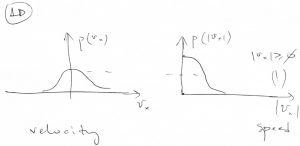
(64) $\begin{equation*} p(v) \:=\: 4\pi \left(\frac{\beta m}{2 \pi} \right)^{3/2} \: v^2 e^{-\beta m v^2/2} \end{equation*}$

Compare this with the distribution of speeds in 1D, which is obtained by simply “folding” together the negative and positive wings of the velocity distribution, since both $v$ and $-v$ imply the same speed $|v|$ :

(65) $\begin{equation*} p(v) \:=\: 2 \left(\frac{\beta m}{2 \pi} \right)^{1/2} \: e^{-\beta m v^2/2} \end{equation*}$

Note the 3D speed distribution has a quadratic “hole” at the origin:

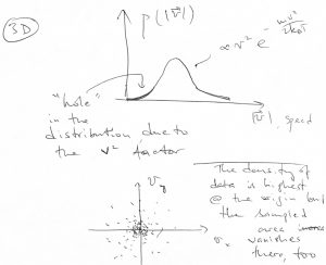
Likewise, the speed distribution will have a linear “hole” of the form $v \, e^{-\beta m v^2/2}$ .

The “hole” comes about despite the value $\vec{v}=0$ being the most likely value of the velocity. There is also a degeneracy of sorts, since in 3D, a whole shell of area $4 \, \pi \, v^2$ contibutes to the same value of $|\vec{v}|$ .

(In 2D, the amount of degeneracy goes with the ring length $2 \, \pi \, v$ .)

Bonus discussion:

There is a rather vivid way to derive the Boltzmann distribution. Imagine a gas subject to gravity:

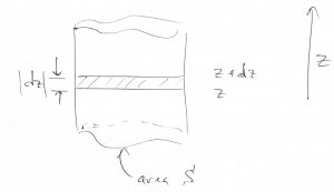
On the one hand, the pressure difference between the altitudes $z$ and $z+dz$ should be exactly compensated by the weight of the gas contained within the layer:

$p(z)\:-\:p(z+dz) \:=\: \frac{m \: g \: n \: S \: dz}{S} \:=\: m \: n\: g \: dz$

where $S dz$ is the volume of the shaded region. Dividing by $dz$ and taking the $dz\to0$ limit yields

$\frac{dp}{dz}\:=\: -m n g$

Yet according to the ideal gas law $p\:=\:n k_B T$ , and so

$\frac{dn}{dz}\:=\:-\frac{nmg}{k_B T}$

Solving the differential equation yields:

$n(z) \:=\: n(z)|_{z=0} \:e^{-\frac{mgz}{k_B T}}$

.

Lastly, we have seen that there are two ways to think about thermal phenomena. Mathematicians prefer to think in terms of probabilities. When two events are uncorrelated, the probability of the compound event factorizes: $p = p_1 \times p_2$ . Chemists and physicists often prefer to think in terms of energies or energy-like quantities. In this case, statistical independence, or lack of interaction between events reveals itself through additivity of energies. The two ways are essentially equivalent, the connection understood through the properties of the mathematical functions $e^x$ and $\ln x$ : $p = p_1 \times p_2 \propto e^{-\beta (E_1 + E_2)}$ or, equivalently, $E=E_1+E_2=-k_B T(\ln p_1+\ln p_2) + \text{const} =-k_B T \ln(p_1 \times p_2) + \text{const} =-k_B T \ln p + \text{const}$ .

License

Icon for the Creative Commons Attribution-NonCommercial-NoDerivatives 4.0 International License

Basic Notions of Thermodynamics and Quantum Mechanics for Natural Sciences Copyright © 2020 by Vassiliy Lubchenko is licensed under a Creative Commons Attribution-NonCommercial-NoDerivatives 4.0 International License, except where otherwise noted.

License

Share This Book