Phase Transitions

Vassiliy Lubchenko

7 Phase Transitions

We have so far dealt largely with systems whose free energy has just one minimum. Changing the volume and/or energy of a system with just one minimum is much like compressing/stretching a mechanical spring. The length and the tension of the spring may change in the process, yet microscopically, the material is much the same as in the absence of external load and will return back to its initial state once the load is off. Consistent with this notion, a thermodynamic state corresponds to a vast set of rather similar microstates that are explored as the system fluctuates. These fluctuations are thus intrinsic physically but are also inherent to the very definition of a thermodynamic state. One should not be misled by the fact that the fluctuations of extensive variables are relatively small, for large systems. In reality, local fluctuations of extensive variables such as the energy, volume, etc., are substantial but largely cancel out when added together. For instance, the average of the total energy of a system of size $N$ scales proportionally with $N$ , while the fluctuation of the total energy go only as $\sqrt{N}$ , a much slower function of $N$ . Non-withstanding these fluctuations, the system characterized by a single minimum has only one thermodynamic state, or “phase”, to speak of.

Let us now consider an alternative situation where the pertinent thermodynamic potential has two minima. It will be most practical to consider a reduced form of the thermodynamic potential $\tilde{G}$ from the preceding Chapter, where we leave the volume $V$ as a variable while setting the energy at its likeliest value for each individual value of volume $V$ :

(1) $\begin{equation*} \tilde{G} \:\equiv\: E_\text{mp}(T, V, N) - T S[E_\text{mp}(T,V,N), V, N] + p\, V\end{equation*}$

Physically, this corresponds to a situation where we have thermal equilibrium in place but not the mechanical equilibrium, unless is so happens that the current value $V$ is at the stable minimum of $\tilde{G}$ . Next, we recognize that the first two terms on the r.h.s. of Eq. 1 actually correspond to the equilibrium value of the Helmholtz free energy $A=E_\text{mp}-T S(E_\text{mp}, V)$ , and so

(2) $\begin{equation*} \tilde{G} \:\equiv \: A(V, T, N) + p \, V \end{equation*}$

In full equilibrium, not just thermal equilibrium, the system must reside in the lowest minimum of this function with respect to the variable $V$ . Indeed, optimizing w.r.t. to $V$ leads to an equation we had derived earlier through a somewhat different route:

(3) $\begin{equation*} \frac{\partial }{\partial V}(A+p V) = 0 \:\: \Rightarrow \:\: \left(\frac{\partial A}{\partial V}\right)_{T, N} \:=\: - p \end{equation*}$

We reiterate that in the l.h.s. formula, the pressure $p$ is regarded as fixed by bringing our system in mechanical contact with an environment maintained at pressure $p$ .

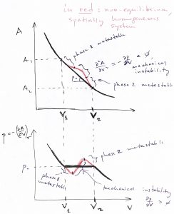
The above equation gives a necessary condition for the function to have an extremum. In addition, we must stipuate that the extremum actually be a minimum, so that the equilibrium is stable. The l.h.s. panel in the figure below illustrates that in this case, fluctuations that cause the volume to decrease subsequently lead to an increase the in the pressure of the system: $\frac{\partial }{\partial V}(A+p_0 V) =-p+p_0<0 \:\Rightarrow\: p > p_0$ , where we denoted the pressure in the environment with $p_0$ to distinguish it from the system’s pressure $p=-(\partial A/\partial V)_T$ , which is equal to $p_0$ only in equilibrium, see Eq. 3. This excess pressure, then, drives the system back to the equilibrium value of the volume, i.e., until $p=p_0$ . Likewise, there is a restoring force toward equilibrium for fluctuations that cause the volume to increase:

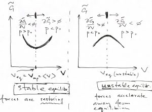
Conversely, an unstable minimum implies that if the system wonders off the equlibrium, it will precipitously continue moving away from the equilibrium, as the r.h.s. panel in the above Figure demonstrates. Indeed, if the volume is less than its value at the maximum, the pressure in the system decreases thus allowing the external pressure to compress the system even further and so on.

In order for the extremum to actually be a minimum, we must require that the second derivative be positive, which, then, implies that the second derivative of the Helmholtz free energy w.r.t. the volume should be positive, too, since the two functions differ only by a linear function of volume, $pV$ , whose 2nd derivative vanishes:

(4) $\begin{equation*} \left( \frac{\partial^2 \tilde{G}}{\partial V^2} \right)_{p, T}\: > \: 0 \: \Rightarrow \: \left( \frac{\partial^2 A}{\partial V^2} \right)_T \: > \: 0 \end{equation*}$

We can use Eq. 3 to further simplify this condition:

(5) $\begin{equation*} \left( \frac{\partial^2 A}{\partial V^2} \right)_T \: = \: \left( \frac{\partial (\partial A/\partial V)_T}{\partial V} \right)_T \: = \: - \left( \frac{\partial p}{\partial V} \right)_T \: > \: 0 \end{equation*}$

Comparing this inequality with the definition of the isothermal compressibility, we conclude the system is mechanically stable, if its isothermal compressibility is positive:

(6) $\begin{equation*} \kappa_T \: > \: 0 \end{equation*}$

which is completely analogous to the earlier established notion that the heat capacity must be positive for the system to be stable w.r.t. thermal fluctuations.

Thus, according to the condition 4, the system is stable if the Helmholtz free energy, as a function of $V$ , is concave up throughout. This insures that the function $\tilde{G}$ has only one minimum and that there is only one thermodynamic states to speak of, as we discussed in the beginning.

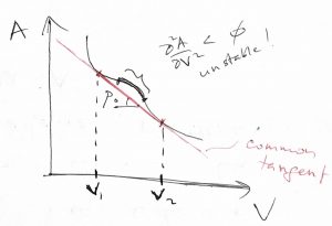
Conversely, if $A(V)$ has a convex–up portion, we expect that a certain subset of microstates become inaccessible, since they correspond to mechanically unstable configurations:

Here and until further notice, we will be working at constant temperature:

(7) $\begin{equation*} T \:=\: \text{const} \end{equation*}$

The region of negative curvature in the above figure separates two regions of positive curvature. In other words, the set of inaccessible configurations in the Figure above—i.e. the $(\partial^2 A/\partial V^2)_T<0$ portion—separate two sets of physically realizable configurations—i.e. the two $(\partial^2 A/\partial V^2)_T>0$ portions—each set corresponding to a thermodynamic state. These two accessible thermodynamic states are distinct in this formal sense and, generally, exhibit distinct physical properties as well, as we will observe later. As such, we regard such distinct thermodynamic states are distinct phases. If the common tangent to the $A(V)$ curve above has the slope $(-p_0)$ , we can readily convince ourselves that one can drive the system to the low volume phase (phase 1) by applying external pressure in excess of $p_0$ and vice versa for the high volume phase:

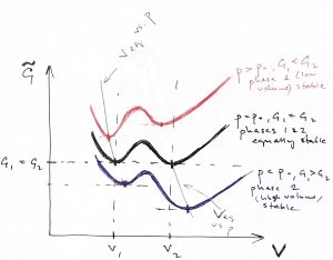
According to the Figure above, if one maintains a fixed pressure $p<p_0$ , the system will spontaneously relax to the high-volume phase while for $p>p_0$ , the system will spontaneously relax to the low-volume phase. Only when $p=p_0$ do the two phases become equally stable, and so the system will relax to one or the other state depending on which side of the col separating the two minima it is prepared. It is instructive to graph the resulting pressure dependence of the equilibrium volume:

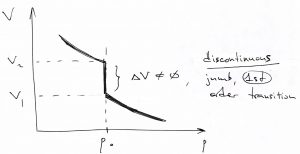
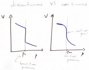
This is a remarkable result! The volume exhibits a discontinuous jump at a particular value of pressure. We call such remarkable situations phase transitions. Specifically, when the relevant control parameter experiences a discrete jump like the one above, we call such transitions discontinuous. A common, though dated, term for such discontinuous phase transitions is the 1st order transition, the word “1st order” referring to the fact the 1st derivative of the free energy w.r.t. to the driving force of the transition (pressure in this case), exhibits a discontinuity.

Since the minimum value of the $\tilde{G}$ function is the equilibrium value of the Gibbs free energy, we conclude that the Gibbs free energies of phase 1 and phase 2 are mutually equal when the two phases are in equilibrium, since the corresponding two minima are exactly of the same depth at the transition:

(8) $\begin{equation*} G_1 \:=\: G_2 \text{ or } \Delta G \:=\: 0 \end{equation*}$

In view of $G=\mu N$ , this implies that the chemical potentials of the two phases are, in fact, equal as well:

(9) $\begin{equation*} \mu_1 \:=\: \mu_2 \end{equation*}$

We reiterate that the above equation embodies the condition that the two phases are in equilibrium w.r.t. particle exchange. (If one phase is more stable than the other, then the stable phase has a lower chemical potential, as should be clear from the Figure above.) The condition in Eq. 9 supplements the other two equilibrium conditions that we had imposed by construction:

(10) $\begin{align*} T_1 \:=\: T_2 \\ p_1 \:=\: p_2 \end{align*}$

the first one taking care of thermal equilibrium and the second one of mechanical equilibrium.

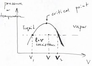
In many cases and, specifically for the vapor—liquid transition, we control not the pressure but the total volume of the system. In this case, the system cannot convert between the phases all at the same time if the total volume is made to change continuously. Instead, the system will convert locally, so that the new phase occupies a progressively larger portion of the space. And so the continuity of the total volume, despite the discontinuity in the volumes of the individual phases, in realized through the continuity of the mole fractions of the two phases. We illustrate this state of affairs using the vapor—liquid transition as an example:

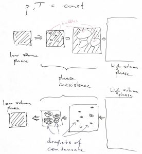
Suppose that during such phase coexistence (during which the two phases literally spatially coexist in one volume) the mole fraction of phase 1 is $x_1$ and the mole fraction of phase 2 is $x_2$ . ( $x_1+x_2=1$ , of course.) Then, the total volume of the system is just the volume that the system would have if it were in pure phase 1, times the mole fraction of phase 1, plus the same thing for phase 2:

(11) $\begin{equation*} V\:=\: x_1 \, V_1 \:+\: x_2 \, V_2 \:=\: x_1 \, V_1 \:+\: (1-x_1) \, V_2 \end{equation*}$

Here we ignore the volume of the interface spatially separating the two phases. The intreface width is usually very small, in which case the volume of such and interfacial region is much smaller than the volume of either of the pure phases. By the same token, the total free energy is

(12) $\begin{equation*} A\:=\: x_1 \, A_1 \:+\: (1-x_1) \, A_2 \end{equation*}$

Eliminating $x_1$ from the two equations above yields that for a phase separated system—which is the equilibrium configuration for $V_1 < V < V_2$ —the free energy depends linearly on the total volume $V$ :

(13) $\begin{equation*} A\:=\: \frac{V_2-V}{V_2-V_1} A_1 \:+\: \frac{V-V_1}{V_2-V_1} A_2 \end{equation*}$

We show this in the Figure below. Consistent with the 2nd Law, the equilibrium value of the free energy (solid black line) is less than the non-equilibrium value (red line), which the system would have if it remained spatially homogeneous:

Alongside we also showed the corresponding dependence of the pressure on the volume, again at constant temperature. Such curves are called isotherms. One should recognize that the isotherm shown above is the same as the $V$ vs. $p$ curve shown earlier, but the graph is now “flipped” so that $V$ is now the horizontal axis and $p$ is the vertical axis.

The equilibrium isotherm directly shows that once phase separation begins, the systems remains at constant pressure and temperature until it is fully converted to the other phase. We note that in order for a clean liquid to begin to develop bubbles, it must be somewhat over-dilated and/or over-heated. In other words, one must decrease the pressure somewhat below the pressure $p_0$ and/or heat the liquid somewhat above the equilibrium boiling temperature. Likewise, in order for the vapor to begin condensing, it must be somewhat cooled below the equilibrium boiling temperature and/or somewhat compressed beyond the pressure at which the vapor and liquid would co-exist at the temperature in question. This is because of the interfacial regions we mentioned in passing earlier. In the very beginning of the phase-to-phase conversion, the amount of interfacial matter relative to the amount of the new (“minority”) phase is actually not small. At the same time, there is a free energy cost associated with the system beong uniform at volume $V$ such that $V_1<V<V_2$ , per Fig. 6. (The free energy of the spatially-uniform, non-equilibrium branch is higher than that of the equilibrium, phase-separated branch.) As a result, some extra stabilization of the minority phase is needed to compensate for the free energy cost of creating the interface. In practice, nucleation of the minority phase is often facilitated by impurities, dirt, and roughness of the container walls, etc.

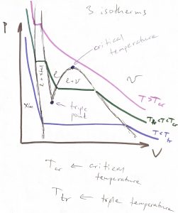
The vapor-liquid transition is special in that the volume discontinuity tends to decrease with the temperature of the transition and, in fact, vanishes at the so called critical point. We illustrate this below using isotherms for three select values of the temperature: below, at, and above the critical temperature:

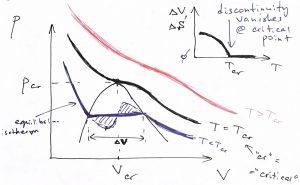
At the critical point, the pressure dependence of the volume still has a divergent derivative but, nonetheless, remains continuous:

As illustrated in Fig.7 , to each temperature there corresponds a unique value of pressure at which vapor-liquid coexistence will be observed. (This pressure grows monotonically with temperature, as we will see shortly.) Thus, one could similarly draw a set of isobars, as see also below. In either case, it is instructive to show the volumes of the pure phases in one graph for a range of temperature or pressure, as we illustrate below:

The volumes $V_1$ and $V_2$ depend on the pressure (temperature). There is one-to-one correspondence between the total volume of a phase-separated system and the mole fraction of the two phases, as we have already seen in Eq. 11. We re-write this equation in a slightly different form, which is known as the lever rule:

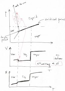
(14) $\begin{equation*} \frac{x_2}{x_1} \:=\: \frac{V-V_1}{V_2-V} \end{equation*}$

Now, what happens to the liquid or gas if one continues to lower temperature and/or pressure? A common scenario is that both will eventually convert into a crystalline solid, as we illustrate in the figure below, where we show three kinds of coexistences in one diagram: liquid-Xtal, liquid-vapor, and Xtal-vapor:

The three isotherms in the figure above can also be shown on a $p-T$ phase diagram, where they become straight lines, as below:

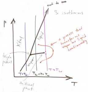
As a bonus feature, we showed above a process, using an orange curve, that takes one between the vapor and liquid state without crossing the phase boundary. This is a unique consequence of the liquid-vapor transition where the phase boundary ends at a finite temperature—thus resulting in a critical point—and signifying that the vapor and liquid are fundamentally equivalent phases. Namely, these are phases where the particles are allowed to freely translate on the experimental time scale.

Just as well, one can perform constant pressure experiments:

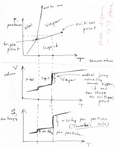
We see that for sufficiently low pressures a gas can turn into a solid bypassing the liquid state. The volume changes for the gas-crystal and gas-liquid transitions can be arbitrarily large. (The volume change for the gas-liquid transition can be small, but this is seen only close enough to the critical point.) In contrast, the entropy changes for such transitions seem vary less from substance to substance. And so, for instance the entropy change for the liquid-to-vapor transition is numerically close to $10 \, k_B$ per particle:

(15) $\begin{equation*}\Delta s_\text{evaporation} \: \simeq \: 10 \, k_B \end{equation*}$

which is known as Trouton’s Rule. This rule may seem arbitrary but it is not. It comes about because at and near normal conditions—which are pertinent to human activities—most gases of practical interest are dilute. In fact, we have seen in one of our homework exercises that the volume increase resulting from evaporation of water is about a factor of thousand. Thus the entropy increase can be estimated as $k_B \ln (10^3) \approx 7 k_B$ per particle, semi-quantitatively consistent with Trouton’s rule. Conversely, Trouton’s rule breaks down close to the critical point, where the entropy change must vanish, see also below.

The entropy of melting is also quite consistent among different substances and is always on the order of $1 \, k_B$ per particle, usually numerically close to $1.5 \, k_B$ , but could be larger for large molecules:

(16) $\begin{equation*}\Delta s_\text{melting} \: \simeq \: 10^0 \, k_B \end{equation*}$

A number of substances, some of which are extraordinarily important, exhibit the interesting property that their volume actually decreases when they melt, while the corresponding phase boundary on the $(p, T)$ has a negative slope. These important substances include water and elemental silicon and germanium.

At the same time, the entropy always increases during a transition driven by heating the system. We can use Thermodynamics to understand this. First, let us sketch the Gibbs free free energy per particle, i.e. the chemical potential, for both phases as functions of temperature:

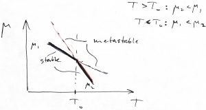
The stable phase is the one with the lower value of $\mu$ , and so according to the above Figure, phase 1 is the low temperature phase and phase 2 is the high-temperature phase. For geometrical reasons, the (negative) slope of the $\mu_2(T)$ dependence should be greater than the (negative) slope of the $\mu_1(T)$ dependence, as the picture above demonstrates. And so,

(17) $\begin{equation*} -\left. \left(\frac{\partial \mu_2 }{\partial T } \right)_p \right|_{T=T_0} \:>\: -\left. \left(\frac{\partial \mu_1 }{\partial T } \right)_p \right|_{T=T_0} \end{equation*}$

But according to the Gibbs-Duhem equation, $d\mu = -sdT+vdp$ , we have $-(\partial \mu/\partial T)_p = s$ , i.e., the entropy per particle. Thus we obtain that the entropy always increases for a transition from a low-temperature phase to a high-temperature phase: $s_2(T_0) > s_1 (T_0)$ , or,

(18) $\begin{equation*}\Delta S \:>\: 0 \text{ for low-T to high-T phase transition} \end{equation*}$

This is natural. Indeed, as one increases the temperature or, at least, attempts to increase the temperature, one must put heat into the system. In fact, we can use Eq. 8, $0=\Delta G=\Delta(H-TS)=\Delta H-T \Delta S$ , to show that the enthalpy of the transition is simply the entropy of the transition times the temperature:

(19) $\begin{equation*} \Delta H \: = \: T\Delta S \end{equation*}$

which, again, is always positive for a transition driven by heating. We note that the temperature staying constant during the phase transformation is an example of the Le Chatelier principle, which states that the system will respond to an external perturbation so as to minimize the effect of the perturbation. Indeed, the absorbed heat goes toward phase transformation, as if the system resisted to our attempts to increase its temperature.

Note that the converse is also true: During a transition from the higher-temperature to the low-temperature phase, heat will be released.

Because the temperature stays constant during phase transformations, one defines the specific heat of the transition per some unit of the substance such as mass or mole.

Transitions driven by changing the pressure have an analogous property: The high pressure phase will always have a lower volume than the low pressure phase. Indeed, according to the Gibbs-Duhem equation, $(\partial \mu/\partial p)_T = v$ , $v$ being the specific volume. This is, again, an instance of the Le Chatelier principle. Note that because the volume of water is lower than that of ice, one can actually induce melting by compressing ice. And incredibly important consequence of the fact that ice is lighter than water is that the bottom of the ocean does not solidify despite the humongous pressure due to the water mass above it. This allows for a great thickness of the ocean and was, likely, essential for the preponderance of early water organisms that produced oxygen, which, then, allowed for more complex life forms. For the same reason, fresh water lakes and rivers freeze near the surface—the ice does not sink because it is lighter—and so deep lakes and rivers do not freeze through during the winter. This allows complex organisms living in those reservoirs and whose life cycles exceed one year to survive the winter.

Now in contrast with entropy, the volume change during a transition caused by heating or cooling could be of either sign, as we have already seen. Microscopically, this can be caused by a variety of reasons. For instance, water ice or crystalline silicon are characterized by highly directional bonding resulting in rather open structures. When these open structures melt, the bonds partially break causing the coordination number to actually increase, which, then, causes a decrease in volume. Let us show that the sign of the volume change determines the slope of the corresponding phase boundary on the pressure-temperature plane. Indeed, consider a small increment of the temperature while moving along one side of the boundary and along the other side of the boundary, respectively:

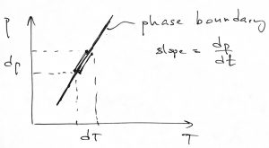
For these two processes, we can write the Gibbs-Duhem equation for the corresponding increment in the chemical potential:

(20) $\begin{align*} d \mu_1 \:=\: -s_1 \,dT\:+\: v_1\, dp \\ d \mu_2 \:=\: -s_2 \, dT\:+\: v_2 \, dp \end{align*}$

where indices 1 and 2 refer to the two sides of the phase boundary. Next we note that the chemical potentials on the opposite sides of the phase boundary are always mutually equal. This implies that $d \mu_1 = d \mu_2$ . Subtracting the two equations above from each other gives the following simple expression for the slope of the phase boundary:

(21) $\begin{equation*} \frac{dp}{dT} \:=\: \frac{\Delta s}{\Delta v} \end{equation*}$

where $\Delta s$ and $\Delta v$ are the entropy and volume changes for the transition at the pressure and temperature in quesion. One must be consistent in computing these changes. For instance, if $\Delta s=s_2-s_1$ , then $\Delta v = v_2-v_1$ . Conversely, if $\Delta s=s_1-s_2$ , then $\Delta v = v_1-v_2$ .

The above equation is known as the Clausius-Clapeyron equation. It can be written in a variety of forms. For instance, one can use Eq. 19 to write it as

(22) $\begin{equation*} \frac{dp}{dT} \:=\: \frac{\Delta h}{T \Delta v} \end{equation*}$

where $\Delta h$ is the enthalpy of the transition per particle. Note that because both the enthalpy and volume are extensive variables, we can re-write the r.h.s. in a variety of ways while being mindful that both the enthalpy and volume must be given per the same unit of matter, be it a mole or kilogram, or whatnot.

According to Eq. 21, for transitions that are driven by heating, $\Delta s > 0$ , but exhibit a negative volume change, $\Delta v<0$ , the slope $dp/dT$ must be negative, as is the case experimentally.

Eq. 21 also helps understand why the slope of the liquid-Xtal boundary is steeper than the slope of the liquid-vapor boundary. Indeed, despite the greater value of $\Delta s_\text{vaporization}$ , relative to $\Delta s_\text{melting}$ , the volume changes accompanying vaporization are even greater. Recall that the specific volume of a gas at normal conditions is roughly three orders of magnitude greater than that of the corresponding liquid. As a result the quantity $\Delta s/\Delta v$ is always smaller for the liquid-to-vapor than the crystal-to-liquid transtion.

There are different kinds of phase diagrams. As a useful example, we provide the pressure-temperature diagram, but with axes flipped so that the pressure is now the horizontal axis, and, alongside, the corresponding diagram where the horizontal axis is the concentration. The latter one is quite a bit more informative as it gives a better sense of phase coexistence:

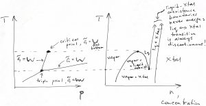
The so called triple point is the point on the phase diagram where the three phase boundaries—liquid-vapor, liquid-Xtal, and vapor-Xtal, respectively—cross. A single-component substance can have at most one triple point (Gibbs phase rule). The $\tilde{G}$ function has three minima at the triple point. In general, already a pure substance can a very substantial number of phases. Phase diagrams of mixtures can become mind-bogglingly complex. In addition, there is still a possibility that there is phase that is not stable under any conditions but can be kinetically accessible. These rich phenomena are subject of Materials Science.

Finally, we can use Eq. 8 and the relation between the Gibbs and Helmholtz free energy, $G=A+pV$ , to relate the Helmholtz free energy change during the transition to the corresponding volume change:

(23) $\begin{equation*} \Delta G = \Delta (A+pV)=0 \: \Rightarrow \: \Delta A= -p \, \Delta V \end{equation*}$

We observe that the Helmholtz free energy always decreases for a transition incurring a volume increase. Moreover, the magnitude of this decrease is exactly equal to the work needed to expand the system to the new value of the volume. This is consistent with our earlier conclusion that the amount of mechanical work one can extract at constant temperature should match the decrease of the Helmholtz free energy.

The above equation should have been obvious already from Figure 6, where, we see, $p_0 = -\frac{A_2-A_1}{V_2-V_1} = -\frac{\Delta A}{\Delta V}$ . There is a useful consequence of this fact. Indeed, we just established that

(24) $\begin{equation*} A_2 - A_1 = -p_0 (V_2-V_1) \end{equation*}$

One the other hand, since $p = -(\partial A/\partial V)$ for the non-equilibrium isotherm,

(25) $\begin{equation*} A_2 - A_1 = -\int_{V_1}^{V_2} p \, d V \end{equation*}$

Thus the areas under the equilibrium and non-equilibrium isotherms, in the $[V_1, V_2]$ interval, are exactly equal to each other. This implies that the two shaded regions in Fig. 7 must have the same area, too. This, then, allows one to determine the equilibrium pressure of the transition if a non-equilibrium isotherm is known, without having to explicitly compute the Helmholtz free energy as a function of volume and determining the common tangent. This recipe is known as “the Maxwell construction.”

Advanced Discussion.

The advanced discussion in the preceding Chapter, on the number of thermally available states to a collection of indistinguishable particles, is directly pertinent to the question of the melting entropy. Let us convince ourselves that there is an entropic advantage to the particles being allowed to exchange places in the liquid, as opposed to be each tied to certain locations in a solid. This entropic advantage turns out to account for much of the melting entropy. Other contributions, such as those due to the dependence of the bond enthalpy on details of local coordination, are undoubtedly present. To separate those contributions from the one in question, we assume that in both the liquid and the solid, the total volume available to the particles, call it $V_f$ , is the same. This “free volume” $V_f$ can be thought of, informally, as the total volume minus the excluded volume due to interactions with the rest of the particles, such as steric repulsion or the directionality of chemical bonds. In a liquid, particles exchange places, thus one cannot speak of a particle location that could be used to label the particles. In this way, liquids exhibit symmetry with respect to particle translations and so one must resort to using local density and various other averaged-out quantities to characterize correlations among particle locations. The number of thermally available states in a liquid is $Z_\text{liq} = (V_f/\Lambda_{dB}^3)^N/N!$ , per the discussion in the preceding Chapter, where the factorial $N!$ takes care of the fact that permutations of identical particles do not lead to microscopically distinct configurations. In a solid, in contrast, particles each vibrate around a certain location and thus can be distinguished. Each particle has $V_f/N$ worth of volume available. Consequently, the number of thermally available states is simply the product of the respective numbers for the individual particles: $Z_\text{sol} = (V_f/N \Lambda_{dB}^3)^N$ . The change in the volume-dependent part of the entropy, due to the transition, is $k_B \ln Z_\text{liq} - k_B \ln Z_\text{sol} = k_B \ln (N^N/N!) \approx N k_B$ , where we used the Stirling approximation $\ln n! \approx n \ln n -n$ , ( $n \gg 1$ ). In other words, restoration of translational symmetry, due to melting, leads to an entropy increase on the order of $k_B$ per particle. This is indeed quite close numerically to melting entropies of actual materials.