Bound states. The particle in the box and other quantum-mechanical models. Quantum numbers. Heisenberg’s uncertainty principle. Atoms and Bonding.

Vassiliy Lubchenko

12 Bound states. The particle in the box and other quantum-mechanical models. Quantum numbers. Heisenberg’s uncertainty principle. Atoms and Bonding.

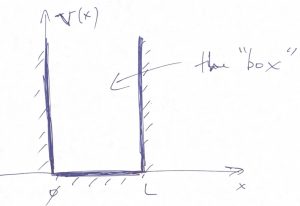
The understanding of how long-lived bound states come about is, arguably, the most important benefit of Quantum Mechanics. To begin the discussion, we start off with the simplest, even if artificial model, where we place our system in a box with infinite walls. Consider a “particle in the box” or square well with infinity walls, whereby the potential energy vanishes inside the box while being infinitely high outside the box:

(1) $\begin{equation*} V(x) = \begin{cases} 0, & 0\:<\:x\:<\:L \\ \infty, & x\:\leq\:0\:\text{and}\:x\:\geq\:L \end{cases} \end{equation*}$

Let us recap the time-independent Schroedinger Equation below:

(2) $\begin{equation*} -\frac{{\hbar}^2}{2m}\frac{{\partial}^2}{\partial{x^2}}\psi(x) \:+\:V(x)\psi(x) \:=\: E \, \psi(x) \end{equation*}$

To be clear, we are looking for finite energy solutions of the Schrodinger equation, which means the r.h.s. must be finite (i.e. not infinite). Since the l.h.s. is thus also finite, we must have it that the wave function must vanish outside the box. Otherwise, the product $V(x) \, \psi(x)$ would be infinite. Thus we have $\psi(x)=0$ for $x \le 0$ and for $x \ge L$ . This fixes the boundary conditions for the values of the wave function at the edges of the box:

(3) $\begin{equation*} \psi(0)\:=\: 0 \end{equation*}$

(4) $\begin{equation*} \psi(L)\:=\:0 \end{equation*}$

Inside the box, the potential energy vanishes, $V(x)=0$ , therefore we have a very simple equation

(5) $\begin{equation*} - \frac{\hbar^2}{2m} \frac{d^2}{dx^2} \: \psi(x) \:=\: E \, \psi(x) \end{equation*}$

Our task is to find all allowed values of the energy $E$ . As we saw in the preceding Chapter, the above equation is solved by a linear combination of the sine and cosine function:

(6) $\begin{equation*} \psi(x)\:=\:C_1 \cos(kx)\:+\:C_2 \sin(kx) \end{equation*}$

Inserting this solution in the l.h.s. of Eq. 5 yileds

(7) $\begin{equation*} - \frac{\hbar^2}{2m} \frac{d^2}{dx^2} [C_1 \cos(kx)\:+\:C_2 \sin(kx) ]\:=\: \frac{\hbar^2 k^2}{2m} [C_1 \cos(kx)\:+\:C_2 \sin(kx) ] \:=\: \frac{\hbar^2 k^2}{2m} \psi(x) \end{equation*}$

Comparing this with the r.h.s. of Eq. 5 immediately yields a connection between the energy eigenvalue $E$ and the wave vector $k$ :

(8) $\begin{equation*} E \:=\: \frac{\hbar^2 k^2}{2m} \end{equation*}$

The boundary condition 3 implies

(9) $\begin{equation*} \psi(0)\:=\:C_1 \cos(0)\:+\:C_2 \sin(0) \:=\: C_1 \:=\: 0 \end{equation*}$

implying the solution is simply the sine function $\psi(x) \propto \sin(kx)$ , where we still need to determine the value of the wave vector $k$ . This is afforded by applying the boundary condition 4:

(10) $\begin{equation*} \psi(L)\:=\: 0 \: \Rightarrow \: C_2 \sin(kL) \:=\: 0 \end{equation*}$

The equation $\sin x = 0$ is solved by any integer multiple of $\pi$ : $x=\pi \, n$ , $n=0, \pm 1, \pm 2, \pm 3, \ldots$ . Therefore we have $kL = \pi \, n \:\Rightarrow \: k=\pi n/L$ . However, the $n=0$ option implies $k=0$ and, hence, $\sin(kx)=\sin(0)=0$ , i.e., no particle at all. Thus $n=0$ is not a valid option. Note further that the $(+n)$ and $(-n)$ options are equivalent. Indeed, a $(-n)$ solution is simply the negative of the corresponding $(+n)$ solution: $\sin(-\pi n/L)=-\sin(\pi n/L)$ . If two solutions differ only by a multiplicative constant, they correspond to the very same microstate and, thus, are equivalent, as we discussed in the preceding Chapter. Thus, only the following values of the wave vector correspond to physically distinct microstates:

(11) $\begin{equation*} k_n \:=\: \frac{\pi \, n}{L}, \hspace{5mm} n=1, 2, 3, \ldots \end{equation*}$

where we used the index $n$ to label the wave vectors corresponding to distinct states. The quantity $n$ is an example of what we call a quantum number. Now that we know the allowed values of the wave vector, we can evaluate the corresponding energy eigenvalues, using Eq. 8:

(12) $\begin{equation*} E_n \:=\: \frac{\hbar^2 k_n^2}{2m}\:=\: \frac{\hbar^2 \pi^2}{2m L^2} \: n^2, \hspace{5mm} n=1, 2, 3, \ldots \end{equation*}$

and the eigenfunction itself, as follows from Eqs. 9 and 10:

(13) $\begin{equation*} \psi_n(x) \:=\: A_n \sin(k_n x) \end{equation*}$

Where $A_n$ is a fixed number, to be determined, and we are relieved to notice that the wave function can be made real-valued, since nothing prevents us from choosing the normalization constant to be real-valued. It is a general pattern that one always may—but does not have to!—choose the wave function of a bound state to be real-valued. To fix the value of $A_n$ , we must specify the number of particles. Here we choose exactly one particle, for concreteness, and so for any $\psi(x)$ :

(14) $\begin{equation*} \int_0^L p(x) \, dx \:=\: \int_0^L |\psi(x)|^2 \, dx \:=\: \int_0^L \psi^2(x) \, dx \:=\: 1 \end{equation*}$

where use the fact that our wavefunctions are real-valued and, so, $\psi^*(x)=\psi(x) \: \Rightarrow \: |\psi(x)|^2 =\psi^2(x)$ . Thus for $\psi(x)=\psi_n(x)$ , it must be true that

(15) $\begin{equation*} A_n^2 \int_0^L \sin^2 \left(\frac{\pi n x}{L}\right) \, dx \:=\: 1 \end{equation*}$

We can easily check, using the formula $\sin^2 x = (1-\cos 2x)/2$ that the integral above is equal to $L/2$ irrespective of the value of $n$ , and so $C_2=(2/L)^{1/2}$ . This yields

(16) $\begin{equation*} \psi_n(x) \:=\: \left(\frac{2}{L}\right)^{1/2}\sin \left(\frac{\pi n x}{L}\right) \end{equation*}$

We graphically summarize these results below, where we show several low energy states and, on the side sketch the corresponding wave functions. The lowest energy state is called the ground state, the 2nd lowest energy state “the 1st excited state”, and so on:

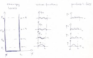
We notice an important pattern that the wave function at the lowest energy is an even function w.r.t. reflection around the center of the well, while the next one is an odd function w.r.t. that reflection implying, then, that the wavefunction should have a node in the middle. The next energy state, again has an even eigenfunction, and so on. This important alternation pattern comes about because the potential energy $V(x)$ is symmetric with respect to reflection about a certain point in space.To understand this, it is convenient to place the origin into that special point. In the so chosen reference frame, the symmetry of the potential can be expressed mathematically as follows:

(17) $\begin{equation*} V(x) \:=\: V(-x) \end{equation*}$

In other words, the potential is an even function of its argument. Below, we exemplify both an even and odd function, for future reference:

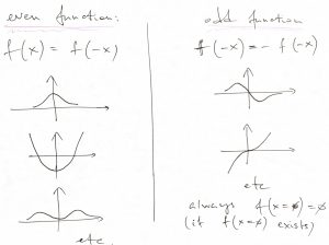
Note that an odd function must always vanish at the origin, because and odd function is the negative of itself at the origin: $f(0)=-f(-0)=-f(0)$ , which, then, implies $f(0)=0$ .

Now, take the time-independent Schroedinger Eqn:

(18) $\begin{equation*} -\frac{{\hbar}^2}{2m}\frac{d^2}{dx^2}\psi(x) \:+\:V(x)\psi(x) \:=\: E \, \psi(x) \end{equation*}$

and replace the argument $x$ by its negative $-x$ :

(19) $\begin{equation*} -\frac{{\hbar}^2}{2m}\frac{d^2}{(d (-x))^2}\psi(-x) \:+\:V(-x)\psi(-x) \:=\: E \, \psi(-x) \end{equation*}$

which amount to swapping the labels “positive” and “negative” for the directions in space. No actual changes to the system are inflicted. Since $(d (-x))^2 = (-d x)^2= (d x)^2$ and $V(x) \:=\: V(-x)$ , we obtain that the function $\psi(-x)$ obeys the same equation as the function $\psi(x)$ :

(20) $\begin{equation*} -\frac{{\hbar}^2}{2m}\frac{d^2}{d x^2}\psi(-x) \:+\:V(x)\psi(-x) \:=\: E \, \psi(-x) \end{equation*}$

On the other hand, since our relabeling of the direction in space did not create a distinct physical state, the “new” solution must be equal to the old one, up to a multiplicative constant:

(21) $\begin{equation*} \psi(-x) \:=\: C \, \psi(x) \end{equation*}$

and, likewise,

(22) $\begin{equation*} \psi(x) \:=\: C \, \psi(-x) \end{equation*}$

Substituting one of the two equations above into the other immediately yields:

(23) $\begin{equation*} C^2 \:=\: 1 \end{equation*}$

or,

(24) $\begin{equation*} C \:=\: \pm \, 1 \end{equation*}$

The $+1$ option implies the wave function is even: $\psi(x)=\psi(-x)$ , while the $-1$ option implies the wave function is odd: $\psi(x)=-\psi(-x)$ . To summarize, we have established that the wave function of a state bound inside a potential energy that’s an even function must be, itself, either even or odd. These ideas can be extended to other types of symmetry, such as those w.r.t. rotation around an axis, as in the molecule of benzene, or spatial translations, as in periodic crystals.

In addition to the aforementioned alternation in the parity of the wave-function, we also notice that for each next energy level, we get an additional node and an oscillation to the wavefunction, which is a general pattern.

According to Eqs. 11 and 12, both the momentum and energy of distinct microstates of a particle confined to a box are quantized. In other words, the momentum and energy of distinct microstates take values that are not continuously distributed but, instead, form a discrete set. The remarkable fact comes about, formally, because the wave function must vanish at the boundaries of the box. One can also think of the wave function as a standing wave (see the end of the last Chapter). In order for a wave to be standing, the size of the box must match an integer number of half-periods of the wave, c.f. Eq. 11.

Despite being a gross approximation, the particle in the box yields a really important pattern, namely, that the energy cost of confining, or, localizing the motion of a particle to an interval of finite length $L$ in any spatial direction follows the following trend:

(25) $\begin{equation*} E_\text{kin} = \frac{p^2}{2m} \sim \frac{\hbar^2 n^2}{m L^2} \end{equation*}$

Various phenomena, such as the existence of metals and the circular shape of the benzene ring, ultimately come about because the electrons holding together those objects have minimized their kinetic energy by delocalizing over the whole system. More specifically, the only non-zero component of the energy of the particle in the box is the kinetic energy, as we have indicated with the label “kin”. Thus we conclude that by spatially “spreading” as much as possible, subject to the potential energy, the particle minimizes its kinetic energy.

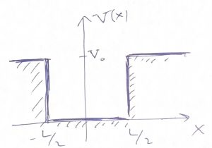
The two main idealizations of the particle in box are that the potential (a) is too tall outside of the box and (b) is too steep. Let us address the first idealization by considering a box whose walls are of finite height $V_0$ , while the width is $L$ as before:

(26) $\begin{equation*} V(x)\:=\: \begin{cases} 0, & -L/2 \:<\:x\:<\: L/2 \\ V_0, &x\:\le \: -L/2\: \text{ or } \:x\: \ge \: L/2 \end{cases} \end{equation*}$

It is somewhat more convenient to center the potential well at the origin:

Inside the well, where $V(x)=0$ , the Schroedinger equation reads

(27) $\begin{equation*} -\frac{\hbar^2}{2m}\frac{d^2}{dx^2}\, \psi_n \:=\: E_n \psi_n \end{equation*}$

while outside, where $V(x)=V_0$ , we have

(28) $\begin{equation*} -\frac{\hbar^2}{2m}\frac{d^2}{dx^2}\, \psi_n \:+\: V_0 \, \psi_n \:=\: E_n \psi_n \end{equation*}$

The energy of the particle cannot have negative values since $V(x) \ge 0$ everywhere in space, while the kinetic energy must be positive at least somewhere. Thus we observe that just like in the above case of the infinitely deep well, the solutions inside the well are oscillating functions of the coordinate. Still, there is the difference that the wave function no longer vanishes at the edges of the well, since $V(x)$ is finite there. The eigenfunctions must be either even or odd functions, as already discussed, while we know that the cosine is an even function while the sine is an odd function w.r.t. reflection about the origin. Thus we infer, by symmetry, that the ground state must be a cosine function:

(29) $\begin{equation*} \psi_1(x) \:=\: C_1 \, \cos(k_1 \, x) \end{equation*}$

the first excited state is a sine function:

(30) $\begin{equation*} \psi_2(x) \:=\: C_2 \, \sin(k_2 \, x) \end{equation*}$

and so forth. Inserting these Eq. 27 implies that, as in the case of the infinitely deep well, we have

(31) $\begin{equation*} E_n \:=\: \frac{\hbar^2 k_n^2}{2m}, \hspace{5mm} n=1, 2, 3, \ldots \end{equation*}$

however the quantization conditions for the wave vector $k_n$ are similar but no longer as simple as in Eq. 11, nor are the conditions for the normalization constants $C_n$ because the wave function does not vanish outside the well. In any event, the earlier made notions regarding the symmetry of the wavefunctions and the number of nodes inside the well still hold.

How does the wave function behave outside the well? Here we have two options. For $E_n < V_0$ , Eq. 32 gives an eigenvalue problem where the eigevalue is now negative:

(32) $\begin{equation*} -\frac{\hbar^2}{2m}\frac{d^2}{dx^2}\, \psi_n \:=\: (E_n-V_0) \psi_n \end{equation*}$

This equation is solved not by a combination of sine and cosine functions but, instead, by the usual exponential function: $e^{+\kappa_n x}$ or $e^{-\kappa_n x}$ . Inserting these into Eq. 32 yields:

(33) $\begin{equation*} \frac{\hbar^2 \kappa_n^2}{2m} \:=\: (V_0-E_n) \end{equation*}$

and, hence,

(34) $\begin{equation*} \kappa_n \:=\: \sqrt{2m (V_0-E_n)}/\hbar \end{equation*}$

where chose $\kappa_n$ to be the positive root for concreteness. To make sure the wave function is normalizable, i.e., we are dealing with a finite number of particle, we must correctly choose which of the two exponentials is used to the right of the well and which one to the left:

(35) $\begin{equation*} \psi_n(x)\:=\:B_n e^{-\kappa_n x}, \hspace{5mm} x>L/2 \end{equation*}$

(36) $\begin{equation*} \psi_n(x)\:=\:D_n e^{+\kappa_n x}, \hspace{5mm} x< -L/2 \end{equation*}$

Thus we obtain that the wave function does not vanish in the region of space where the values of the energy are less than the potential energy! Note that a classical particle would not be able to penetrate regions where the total energy is less than the potential energy because it would cause the kinetic energy to be negative. But the kinetic energy of a classical particle, $mv^2/2$ is an intrinsically non-negative quantity. Though the wavefunction is seen to penetrate that classically-forbidden region, it still decays there rather rapidly, exponentially in fact. We graphically summarize these notions below:

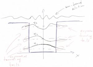
Finally, when the particle’s energy is greater than the highest value of the potential energy: $E_n > V_0$ , the wavefunction becomes wave-like throughout the whole space and, in fact, is best described as a wave packet. The energies values of a wave packet are not quantized but, instead, form a continuum.

The tails of the wavefunction that penetrate the classically forbidden region represent an intrinsically wave-like phenomenon. These tails are often called tunneling tails to signify that the particle can penetrate, or “tunnel” under a potential wall.

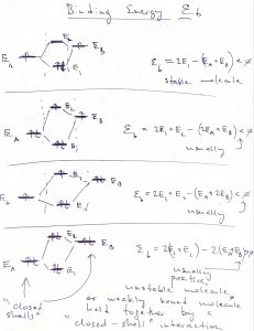
The above example of a potential well with finite walls sets us up for discussing the most basic features of molecular binding. Let us now consider two identical potential wells, each corresponding to the bounding potential of an atom. (Generally, the bounding potential corresponds to a positive nucleus dressed by some electrons that are bound so strongly that they are not affected much by the proximity of other atoms.) In the Figure below, we consider four configurations. The l.h.s. corresponds with the two atoms being far apart, while the r.h.s. with those two atoms being close. Note that we can consider, a priori, a situation where the two atomic wavefunctions (or “orbitals”) have the same sign or have opposite signs. The top of the figure corresponds with the former, “even” possibility, while the bottom of the Figure corresponds with the latter, “odd” possibility:

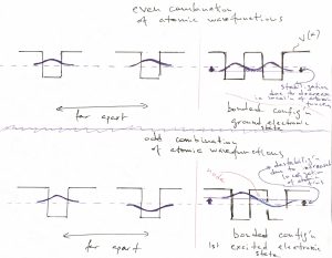
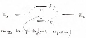
We observe that for the even combination (the top of the Figure), bringing in the other atom allows each of the individual orbitals to extended a little further toward the other atom, because there is now a low energy region available in that direction. As a result, each of the atomic orbitals can lower its kinetic energy, by virtue of Eq. 25. This is in addition to the already mentioned lowering of the potential energy. Hence the overall energy is lowered, too. This stabilization is, ultimately, the origin of the stability of the molecule, relative to the non-bound state, where the atoms are far apart. In more physical terms, this stabilization in the presence of another atom comes about electrons on one atom “feel” the attraction from the other atom and can lower their energy by visiting that part of space, see also below. The odd combination of the atomic function does the opposite thing: Because this combination must have a node and, thus, vanishes in the middle, the individual wavefunctions now extend out less than they would in the absence of the other atom. As a result, both the kinetic energy goes up (the localization length is now somewhat smaller) and the potential energy is not as low because the tunneling tails do not extend toward the low energy regions centered on the other atom. Thus the total energy of this microstate is higher than that of an individual atom, let alone the energy of the binding orbital. This microstate is the first excited state. Below we graphically summarize the above notions of the stabilization/destabilization of the molecular orbitals, relative to the atomic orbitals:

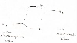
When the two atoms are not identical, the situation is similar in that the ground state orbital is more stable than that on the more electronegative atom while the excited state orbital is less stable than the orbital on the less electronegative atom:

The gap, or “splitting”, between the ground state and 1st excited state of the molecule is a very general phenomenon. We see it comes about because of the possibility of tunneling between bound states, which would not be possible in Classical Mechanics. Because of this splitting, we believe that the ground state of any physical system must be non-degenerate. Indeed, if there were two or more lowest energy states, then the mutual tunneling between these lowest energy states would mix them up and cause one orbital to split off toward lower yet energies. This fact of the uniqueness of the ground state then yields the 3rd Law of Thermodynamics.

We have now most of the ingredients to qualitatively discuss of how the finite size of an atom comes about and the nature of chemical bonding. Below we sketch some of the energy levels and wave functions for the motion of the negatively charged electron in the attractive field of a positively charged nucleus:

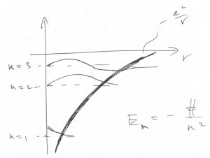
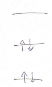
As before, the wave function is a standing wave in the classically allowed region, where the potential energy does not exceed the total energy but decays exponentially in the classically forbidden region. In the simplest way of discussing this, the energy levels form a “ladder” whose steps can accommodate electrons. The electrons possess an internal degree of freedom, called the spin, in addition to the degree of freedom corresponding to the motion in the 3D space. The quantum number for the spin has only two distinct values, corresponding to spin up and down. According to Pauli’s exclusion principle, whose discussion is beyond the scope of this course (but see the bonus discussion at the end), no two electrons can possess the same set of quantum numbers. Thus we can put at most two electrons into one orbital, but only if their spins have distinct values. Thus we can “build” up an atom by placing electrons on the steps of the ladder starting from the lowest energy one:

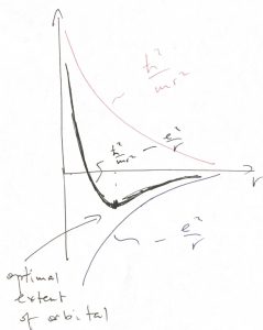
The finite size of an atom comes about for the following reason. On the one hand, the energy of the Coulomb attraction, $V(r)=-e^2/r$ favors the ever closer separations between the electron and the nuclei, since the potential energy is minimized (and, in fact, becomes infinitely negative) as $r \to 0$ . On the other hand, localizing the electron to a region of size $r$ is subject to the penalty of raising the kinetic energy, $\hbar^2/m r^2$ , up to a numerical factor, per Eq. 25. Thus the actual extent of the electronic orbital is controlled by two competing factors and is found by optimizing the total energy $\hbar^2/m r^2-e^2/r$ , which we graphically illustrate below:

To be clear, this is a qualitative argument. One can obtain very accurate solutions for the electronic wave functions in many cases, but the complexity of the solution can obscure the relatively simple meaning of the effect. To summarize, atoms are finite because (a) the orbitals are finite in extent and (b) because one can put at most two electrons in one orbital. As a result, when two atoms come close together, the electrons from one atom cannot jump onto any of the orbitals centered on the other atom, if the latter orbitals are already filled.

They can however jump so if those orbitals are not filled. According to the qualitative picture of the atomic levels mentioned above, those so called “valence” orbitals correspond to less deep energy levels and, at the same time, are more extended than the deep orbitals. It is instructive to sketch the potential felt by a valence electron in the presence of not one, but two nuclei. First, we assume the two nuclei are identical:

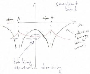
We observe that the ground state orbital is small in the inter-nuclear space because the electron reaches there by tunneling. Despite being small, the wave function is non-vanishing. The corresponding, rather modest amount of negative charge in the inter-nuclear space actually suffices to bind such atoms together. This type of bond is called covalent. It has a characteristic feature of being rather directional, as the bonding electronic density is usually distributed around atoms anisotropically, i.e. not in a spherically-symmetric fashion.

When the two atoms are not identical, then much of the ground state wave function will be centered on the more electronegative atom:

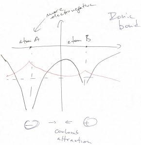
In this case, the valence electrons will flock to the more electronegative atom. As a result, the bond can be well thought of as resulting from Coulomb attraction between a positively and negatively charged objects, both objects exhibiting rather isotropic charge distribution. The resulting type of bond is often referred to as an ionic bond.

The preceding situations are realized when the constituent atoms each contribute an orbital and one electron to the bond. What happens when each atom contributes one orbital that is filled by two electrons? In such cases, neither the covalent bond, nor the ionic bond can realize. Instead, the bond will be of much, weaker nature and results from a mutually induced polarization:

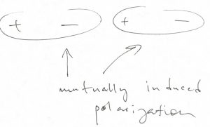
We call such bonds secondary, or closed-shell interactions, the word “closed-shell” referring to the fact that the orbitals in question are filled. The important hydrogen is, formally, an example of a closed-shell interaction and happens to be rather directional because the orbitals involved are rather anisotropic.

The notion of “building up” the atomic orbitals applies to the molecular orbitals as well. We evaluate the energy of an electronic configuration by counting the electrons residing in an orbital and multiplying that by the energy of the orbital:

Again, we remind that at most two electrons can “sit” in one orbital. If the orbital is completely filled, i.e., contains two electrons, the electrons must have oppositely oriented spins. Note we have completely ignored the fact that the energies of the orbitals will generally depend on both the total number of electrons in the system and how they are distributed among the orbitals. These are rather complicated matters that we cannot do justice to in this Course; they are however important and form the subject of Quantum Chemistry.

Finally we touch upon the potential energy of a harmonic oscillator:

(37) $\begin{equation*} V(x) \:=\: \frac{k x^2}{2} \:\equiv\: \frac{m \omega x^2}{2} \end{equation*}$

where $k$ is the spring constant and $\omega \equiv (k/m)^{1/2}$ the oscillator’s frequency. This model is important in Physical Chemistry because it can be used to describe vibrations of chemical bonds. Below we sketch several lowest energy levels alongside the corresponding orbitals:

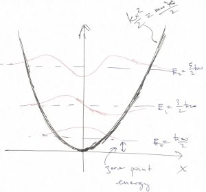
Because the quadratic potential function extends all the way to infinity, all of the states are bound and so the energies of the microstates form a discrete set:

(38) $\begin{equation*} E_n \:=\: \hbar \omega \left(n+\frac{1}{2}\right) \end{equation*}$

As was the case for all the models discussed above, the ground state energy is above the bottom of the potential: $E_0=\frac{\hbar \omega}{2}$ . This “excess” energy is called the zero-point energy and has observable consequences. For instance, it contributes to the formation enthalpy of solids and molecules alike.

Finally, we invoke the notion from Eq. 11 one more time to note that the typical value of momentum of a particle is connected to the size of the region to which the particle is confined

(39) $\begin{equation*} |p| \sim \frac{\hbar n}{L} \end{equation*}$

Since the average momentum is zero—the particle is not going anywhere—this equation can be re-written for the deviation $\delta p$ of the momentum from its average value:

(40) $\begin{equation*} \delta p \sim \frac{\hbar n}{L} \end{equation*}$

At the same time, the box size $L$ can be thought of as the uncertainty $\delta x$ in the position of the particle. Thus we get $\delta p \: \delta x \gtrsim \hbar$ , since $n \ge 1$ . A more accurate estimate is

(41) $\begin{equation*} \delta p \: \delta x \ge \hbar/2 \end{equation*}$

and is known as Heisenberg’s uncertainty principle. It is yet another way of discussing the wave-like nature of what may seem like a particle when experimental resolution is lacking.

Bonus discussion: We also notice the remarkable property of the eigenfunctions of our Hamiltonian that:

(42) $\begin{equation*} \int_0^L \psi_m(x) \, \psi_n(x) \, dx \:=\: \begin{cases} 1, & \text{ if } m=n \\ 0, & \text{ if } m \ne n \end{cases} \end{equation*}$

This is a general pattern that makes it easy to see that one may combine more than one eigenstate of the Hamiltonian to put together an infinite variety of wavefunctions for our system:

(43) $\begin{equation*} \psi(x) \:=\: \sum_n B_n \, \psi_n(x) \end{equation*}$

where the summation is over the quantum number $n$ , which is $n=1, 2, 3, \ldots$ in this specific case, and the constants $B_n$ must be chosen to preserve the normalization. This notion, then, fleshes out the statement we made in the preceding Chapter that one may present an initial state of a quantum-mechanical system in terms of the harmonics, each of which, then, oscillates with its own frequency.

The aforementioned Pauli exclusion principle is yet another realization of the importance of symmetry effects in Quantum Mechanics. We have already considered a special case where the potential energy for 1D motion is an even function of its argument. In this case we saw that a half of the orbitals must have a node at the origin. Now consider a very different type of symmetry. Imagine two identical particles, whose coordinates are $\vec{r}_1$ and $\vec{r}_2$ , respectively. Each particle is subject to an external potential $V(\vec{r})$ . In addition, the two particles may interact via some interaction potential $V_\text{int}(|\vec{r}_1-\vec{r}_2|)$ that depends only on the mutual distance $|\vec{r}_1-\vec{r}_2|$ . We add these potential energies to the kinetic energies of the two particles to put together the Hamiltonian for this system:

(44) $\begin{equation*} \hat{H}(\vec{r}_1, \vec{r}_2) \:=\: -\frac{\hbar^2}{2m} \nabla^2_1 -\frac{\hbar^2}{2m}\nabla^2_2 \:+\: V(\vec{r}_1) \:+\: V(\vec{r}_2) \:+\: V_\text{int}(|\vec{r}_1-\vec{r}_2|) \end{equation*}$

where $\nabla^2 \equiv \partial^2/\partial x^2+ \partial^2/\partial y^2+ \partial^2/\partial z^2$ is the 3D analog of the second derivative w.r.t. the spatial coordinate. The above Hamiltonian has a special property of being symmetrical w.r.t. the interchange of the particles’s labels: $1 \leftrightarrow 2$ :

(45) $\begin{equation*} \hat{H}(\vec{r}_1, \vec{r}_2) \:=\: \hat{H}(\vec{r}_2, \vec{r}_1)\end{equation*}$

One can now perform steps analogous to those that led to Eqs. 21 and 22 and show that the Schroedinger equation satisfied by the function $\psi(\vec{r}_1, \vec{r}_2)$ :

(46) $\begin{equation*} \hat{H}(\vec{r}_1, \vec{r}_2) \psi(\vec{r}_1, \vec{r}_2) \:=\: E \psi(\vec{r}_1, \vec{r}_2) \end{equation*}$

is equally well satisfied by the function $\psi(\vec{r}_2, \vec{r}_1)$ :

(47) $\begin{equation*} \hat{H}(\vec{r}_1, \vec{r}_2) \psi(\vec{r}_2, \vec{r}_1) \:=\: E \psi(\vec{r}_2, \vec{r}_1) \end{equation*}$

Since relabeling the particles does not correspond to physical changes, we conclude such relabeling will at most lead to the wavefunction being multiplied by a constant factor:

(48) $\begin{equation*} \psi(\vec{r}_1, \vec{r}_2) \:=\: C \, \psi(\vec{r}_2, \vec{r}_1) \end{equation*}$

and, likewise,

(49) $\begin{equation*} \psi(\vec{r}_2, \vec{r}_1) \:=\: C \, \psi(\vec{r}_1, \vec{r}_2) \end{equation*}$

This leads to $C^2 = 1$ , and, consequently, to either

(50) $\begin{equation*} C \:=\: +1 \end{equation*}$

or

(51) $\begin{equation*} C \:=\: - 1 \end{equation*}$

The latter possibility is particularly interesting in that it implies that the wave function changes its sign upon interchanging the particles’ identities:

(52) $\begin{equation*} \psi(\vec{r}_2, \vec{r}_1) \:=\: - \psi(\vec{r}_1, \vec{r}_2) \end{equation*}$

Substituting $\vec{r}_2 = \vec{r}_1 = \vec{r}$ immediately yields that the wave function must have a node, i.e., the chances of finding the particles both at the same place vanish:

(53) $\begin{equation*} \psi(\vec{r}, \vec{r}) \:=\: - \psi(\vec{r}, \vec{r}) \hspace{3mm} \Rightarrow \hspace{3mm} \psi(\vec{r}, \vec{r}) \:=\: 0\end{equation*}$

Informally speaking, particles whose exchange properties fall under the rule 51 cannot be in one spot at the same time! It might not be a priori obvious why it should be so, but there are apparently particles that obey the rule 50 and particles that obey the rule 51. The former case is known as the Bose-Einstein statistics, while the latter case as Fermi-Dirac statistics. The electrons happen to obey the Fermi-Dirac statistics, hence the Pauli exclusion principle. This, as we saw earlier in the Chapter is absolutely necessary for atoms to exist as rigid entities. Indeed, electrons can also have two distinct values of the spin and so one cannot put more than two electrons into an orbital, one electron per distinct value of the spin. Consequently, two filled orbitals will repel from each other thus making atoms rather behave like rather rigid objects. While it is possible to squeeze the orbitals themselves, using high pressures, this comes at a cost of increasing the kinetic energy of the electrons, per Eq. 25.

License

Icon for the Creative Commons Attribution-NonCommercial-NoDerivatives 4.0 International License

Basic Notions of Thermodynamics and Quantum Mechanics for Natural Sciences Copyright © 2020 by Vassiliy Lubchenko is licensed under a Creative Commons Attribution-NonCommercial-NoDerivatives 4.0 International License, except where otherwise noted.

License

Share This Book