The molecular origin of hydrostatic pressure and the notion of flux

Vassiliy Lubchenko

3 The molecular origin of hydrostatic pressure and the notion of flux

Here we discuss how the pressure in a gas or liquid comes about at the molecular level and derive an expression for pressure, which is a macroscopic concept, through quantities pertaining to individual molecules. Pressure is a combined result of many molecules hitting the wall of the container. Despite the intermittent character of the molecular collisions, pressure is steady because the effective force exerted by those colliding molecules on the container’s walls is averaged over a substantial area and over times that greatly exceed the duration of an individual collision.

Consider first an idealized setup where we have a steady stream of particles coming out of a source and hitting a heavy shield attached to a stationary wall. The particles each have mass $m$ , velocity $v$ , while the concentration of the particles in the beam is $n$ :

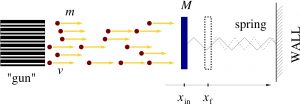
For now, we are interested in a situation where the interactions between the particles are sufficiently weak so that their motions are only weakly correlated, if at all. For the same reason, we will regard the recoiled particles as not interfering in any way with the incoming particles. This argument will eventually lead us to what one calls the ideal gas. The force fluctuates wildly around some average value, as time goes by, and is very messy. Since the individual collisions are uncorrelated, it is convenient to separately consider small patches of the shield such that distinct collisions with each such patch do not overlap temporally. (The forces acting on the distinct patches will be added together at the end of the day.)

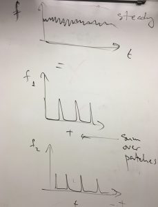
Each of these partial contributions is a temporal sequence of disparate peaks corresponding to individual collisions:

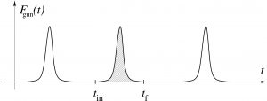
For an individual collision, the particle just begins to touch the shield at time $t_\text{in}$ and stops touching it at time $t_\text{f}$ , while the force peaks out somewhere in-between.

We are dealing here with a force that rapidly changes in time. It spikes during a collision but could be very small at other times. Because the shield is heavy, it will not experience correspondingly rapid fluctuations in its velocity, acceleration, or coordinate. Rather, it will experience a force averaged over a large number of consecutive collisions. Evaluation of this averaged force is, then, a good starting point for the argument, which can be systematically improved upon by including into the treatment deviations of the instantaneous value of the force from its average vale.

Let us estimate the time-averaged force $\langle f \rangle_t$ , where the angular brackets denote averaging over time and, consequently, over the collisions. Perhaps the easiest way to go about this by analogy. Recall how we define the average velocity $\langle v \rangle = \frac{\Delta x}{\Delta t}$ , to be compared with the instantaneous velocity $v = \frac{d x}{d t}$ , where $\Delta x$ is total displacement (i.e., the total increment of the coordinate) over the time interval $\Delta t$ . According to Newton’s 2nd law, the force is the instantaneous rate of change of the momentum, $f = \frac{d P}{d t}$ . Thus the average force $\langle f \rangle = \frac{P_\text{f} - P_\text{in}}{t}$ , where the increment $(P_\text{f} - P_\text{in})$ corresponds to the total momentum imparted to the particle over the time interval $t$ . One can present this total imparted momentum as a sum of contributions due to individual collisions: $P_\text{f} - P_\text{in} = \sum_{k=1}^{N_c} \Delta P_k$ , where $\Delta P_k$ is the momentum imparted during an individual collision labelled with $k$ and $N_c$ is the total number of collisions that occured over time $t$ . Thus we obtain

(1) $\begin{equation*} \langle\:f\:\rangle\:=\: \frac{1}{t} \sum_{k=1}^{N_c} \Delta P_k \:=\: \frac{N_c}{t} \: \frac{1}{N_c} \sum_k^{N_c} \Delta P_k \:=\: \frac{N_c}{t} \: \langle \Delta P \rangle \end{equation*}$

A somewhat more systematic procedure goes like this: First we break up a sufficiently long time interval $[0, t]$ into many very short intervals $\Delta t_i$ such that the force can be regarded as constant over each individual interval. Denote this constant force with $f_i$ . The averaging is, then, reduced to the following weighted average:

(2) $\begin{equation*} \langle\:f\:\rangle\:=\: \sum_i {\frac{\Delta t_i}{t} f_i \end{equation*}$

The averaging above is completely analogous to evaluating, for instance, the average grade in a class where, say, 30% of the students received an A, 50% students received a B, and 20% percent received a C, and so the average grade is $0.30 \times 4 + 0.50 \times 3 + 0.20 \times 2=3.1$ . The $\Delta t_i/t$ ratio plays the role of the weight of the interval $i$ . Note the weights add up to 1, as they should:

(3) $\begin{equation*} \sum_i \frac{\Delta t_i}{t} = \frac{1}{t} \sum_i \Delta t_i = \frac{1}{t} \: t =1 \end{equation*}$

(Note also that in contrast with the class grade example, here two distinct intervals do not have to exhibit distinct values of the force $f_i$ .)

A digression on statistics: In case you forgot how weighted averages come about, it may be worthwhile to review this in some detail. Suppose you have sampled (or measured) a distributed quantity $x$ for a total number of $N$ times. It is often useful to determine the average of this quantity over the sampled data:

(4) $\begin{equation*} \langle x \rangle \equiv \frac{1}{N} \sum_{\alpha=1}^N x_\alpha. \end{equation*}$

Suppose the quantity $x$ can assume any value from an interval $[x_\text{min}, x_\text{max}]$ . We may conveniently subdivide the interval into $M$ small sub-intervals of length $\Delta x$ , so that

(5) $\begin{equation*} \Delta x = \frac{x_\text{max} -x_\text{min}}{M}. \end{equation*}$

Let us label each sub-interval, or “bin”, by integers $1$ through $M$ . Bin $k$ corresponds to the data range $x_\alpha \in [x_k, x_{k+1}]$ . Let us know break up the sum in Eq. (4) into contributions from the distinct bins:

(6) $\begin{equation*} \langle x \rangle = \frac{1}{N} \sum_{k=1}^M \sum_{\text{over bin } k} x_\alpha \end{equation*}$

To avoid confusion, we label the original data using the Greek indices, while the bins are labeled with Latin indices.

Suppose there are $N_k$ data in bin $k$ . One should think of $N_k$ as the height of the bar on a histogram where the width of the bar is the quantity $\Delta x$ itself, such as the one below:

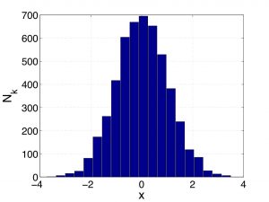
We can conveniently rewrite the equation above as

(7) $\begin{equation*} \langle x \rangle \: = \: \frac{1}{N} \sum_{k=1}^M N_k \:\: \frac{1}{N_k} \sum_{\text{over bin } k} x_\alpha \:=\: \frac{1}{N} \sum_{k=1}^M N_k \:\: x_k \:=\: \sum_{k=1}^M \frac{N_k}{N} \: x_k \end{equation*}$

where $x_k \equiv \frac{1}{N_k} \sum_{\text{over bin } k} x_\alpha$ is the average of the data that falls within bin $k$ . The quantity $x_k$ automatically falls within bin $k$ , too, and can be thought of, approximately, as the position of the center of bin $k$ . This approximation becomes exact in the limit $\Delta x \to 0$ . One may define the statistical weight of bin $k$ :

(8) $\begin{equation*} p_k \equiv \frac{N_k}{N} \end{equation*}$

The weights corresponding to the histogram above are shown below:

These weights obviously add up to unity:

(9) $\begin{equation*} \sum_{k=1}^M p_k = \frac{1}{N} \sum_{k=1}^M N_k = \frac{1}{N} N = 1 \end{equation*}$

c.f. Eq. (3). With the so defined weights $p_k$ , one can now rewrite the average in Eq. (7) in a way that does not explicitly refer to the total size of the data set, but, instead, specifies the fractional amount, or the probability of the outcome $x_k$ , in the total set of all possible outcomes:

(10) $\begin{equation*} \langle x \rangle \: = \: \sum_{k=1}^M p_k x_k \end{equation*}$

Since the weights $p_k$ describe how the probability of encountering the corresponding value of $x$ , they are often called the distribution of the quantity $x$ . End of digression on statistics

Now, in the next step, we take $1/t$ out of the sum in Eq. (2) and take the limit $\Delta t_i \to 0$ , which conveniently yields a definite integral:

(11) $\begin{equation*} \langle\:f\:\rangle\:=\: \frac{1}{t} \lim_{\Delta t_i \to 0} \sum_i {f_i \:\Delta{t_i}} = \frac{1}{t} \int_0^t f(\tau) d\tau \end{equation*}$

We next present the time integral of the force as a sum over distinct peaks corresponding to distinct collisions, in the Figure above. We will use the dummy index $k$ to label distinct collisions:

(12) $\begin{equation*} \langle\:f\:\rangle\:=\: \frac{1}{t} \int_0^t f(\tau) d\tau = \frac{1}{t} \sum_k^{N_c} \int_{t_\text{in}^k}^{t_\text{f}^k} f(\tau) d\tau \end{equation*}$

where $N_c$ is the total number of collisions that occurred over time $t$ . Let us consider an individual integral in the above sum and express the force through the time derivative of the momentum $P$ of the shield, as afforded by Newton’s second law, $f \:=\:\frac{dP}{dt}\:dt$ :

(13) $\begin{equation*} \int_{t_\text{in}}^{t_\text{f}}f\:dt \:=\: \int_{t_\text{in}}^{t_\text{f}} \frac{dP}{dt}\:dt\:=\:\Delta P \end{equation*}$

where $\Delta p$ is thus the momentum change of the shield resulting from an individual collision. Subsequently, one may rewrite Eq. (14) as

(14) $\begin{equation*} \langle\:f\:\rangle\:=\: \frac{1}{t} \sum_k^{N_c} \Delta P_k \:=\: \frac{N_c}{t} \: \frac{1}{N_c} \sum_k^{N_c} \Delta P_k \:=\: \frac{N_c}{t} \: \langle \Delta P \rangle \end{equation*}$

that is, the average force is proportional to the average amount momentum transferred to the shield during an individual collision. The proportionality constant is the collision number $N_c$ divided by the duration $t$ of the experiment. The momentum change, due to a single collision is easily inferred from the last problem we solved in Chapter 2:

(15) $\begin{equation*} \Delta P \:=\: \frac{2mM}{m\:+\:M}\:(v \:-\: v_\text{shield}) \end{equation*}$

where $v_\text{shield}$ is the velocity of the shield just before the collision. We are interested in the steady state result whereby the shield is stationary on the average: $\langle v_\text{shield} \rangle = 0$ . This leads to

(16) $\begin{equation*} \langle \Delta P \rangle \:=\: \frac{2mM}{m\:+\:M}\: v \end{equation*}$

Our next step is to determine the ratio $\frac{N_c}{t}$ .This ratio is, quite literally, the number of particles crossing a surface per unit time, or the collision rate. Evaluation of $N_c$ is done most straightforwardly by going over to the reference frame moving with the particles. In this frame, the particles are stationary, while the shield is moving to the left with the velocity $(-v)$ . The number of particles that collided with the shield over time $t$ in the lab reference frame is, then, equal to the number of particles “swept” by the moving shield in the moving frame.

The figure below shows a slightly more general setup, where the shield is tilted so that the normal to its surface is at angle $\theta$ to the direction of the particle stream:

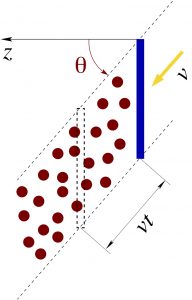
If the area of the shield is $S$ , then the volume swept by the shield over time $t$ is equal to

(17) $\begin{equation*} \text{swept volume} = v \: t \: S \cos \theta \end{equation*}$

To see this, recall that the volume of a (generally oblique) prism is the area of the base of the prism times the distance between the top and bottom bases. Our “prism” has bases of area $S$ each, while the distance between the two planes containing the respective bases is $v \:t \: \cos \theta$ .

The number of particles swept is just swept volume times the particle concentration. Thus

(18) $\begin{equation*} N_c \:=\: n \: v \: t \: S \cos\theta \end{equation*}$

while the rate $N_c/t$ at which particles collide with the shield is

(19) $\begin{equation*} \frac{N_c}{t} \:=\: n \: v \: S \cos\theta \end{equation*}$

This is a useful formula as it allows one to write down a simple result for the particle flux, i.e., the number of particles crossing a surface (real or imaginary) per unit time and unit area:

(20) $\begin{equation*} \text{particle flux: } \:\: J \:=\: \frac{N_c}{t \: S} \:=\: n \: v \: \cos\theta \end{equation*}$

Note that the above formula correctly reflects the fact that if the stream is parallel to the surface ( $\theta=\pi/2$ ), the flux vanishes. Note also that the flux is an intensive property: It does not in any way reflect the size of the system, but only reflects its local properties.

Now let us return to our main derivation. In our particle-shield setup, $\theta=0$ . Hence,

(21) $\begin{equation*} N_c \:=\: n \: v \: t \: S \end{equation*}$

Putting together Eqns. (14), (16), and (21) yields:

(22) $\begin{equation*} \langle\:f\:\rangle\:=\: n \: \frac{2 m M}{m+M} \: v^2 \: S \end{equation*}$

As one could have expected, the total force acting on the shield is proportional to the shield’s area. It is, then, convenient to define the force per unit area, which we call the pressure:

(23) $\begin{equation*} p \: \equiv \: \frac{f}{S} \end{equation*}$

It is an intensive property, i.e., it does not depend on the system size, which, in this case is the size of the shield. Thus one gets:

(24) $\begin{equation*} p \:=\: n \: \frac{2 m M}{m+M} \: v^2 \end{equation*}$

Note a rather general expression we can write down in view of Eqs. (14), (20), and (23):

(25) $\begin{equation*} p \:=\: J \langle \Delta P \rangle \end{equation*}$

which says that pressure, essentially, amounts to a flux of momentum from the incident particles to the object they are colliding with. (More precisely, the hydrostatic pressure is the flux of the normal component of the momentum. There is, generally, also a component of momentum that is parallel to the surface, which will be transferred, if the molecules stick to the walls, even if only transiently. This process actually underlies the phenomenon of viscous response.)

In the important limit of particles being much lighter than the shield, $m \ll M$ , Eq. (24) simplifies and, in fact, contains no reference to the properties of the surface that is being bombarded by our particles:

(26) $\begin{equation*} p \:=\: 2\: n \: m \: v^2 \end{equation*}$

where we used that $mM/(m+M) = m/(1+m/M) \to m$ , as $m/M \to 0$ . Alternatively, one may discuss a pressure on an imaginary, fully stationary surface. In this case, one must assume $M \to \infty$ for consistency. Either way, we obtain that the pressure due to a steady (even if intermittent) stream particles is the property of the particles and the stream themselves and, thus, is of rather universal nature. The concept of pressure will be prove quite useful indeed.

While fully demonstrating the molecular origin of pressure, Eq. (26) must be generalized a bit before we can apply it to actual gases of particles because in equilibrium gases, the velocities of the particles are distributed. Which means that both the speed and the angle of incidence (this is the angle $\theta$ above) are distributed and one must average over those distribution. Setting up the averaging is not too difficult, derivations given in my CHEM4370 notes or any standard texts on Thermodynamics. In short, one should group the incident molecules into streams like the one we have worked with, each stream characterized by a specific value of $v$ and $\theta$ and to remember that the momentum transfer to the shield is determined by the component of the particle’s velocity along the normal to the shield: $\Delta P \to \Delta P \cos\theta$ . Finally, only a half of all particles is moving toward the shield, while the other half is moving away.

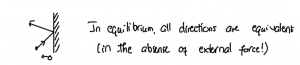
All these complications amount to simply introducing an additional, multiplicative factor $1/6$ into the formula and the necessity to average the speed squared over all particles in the gas:

(27) $\begin{equation*} p \:=\frac{1}{3} \: n \: m \: \langle v^2 \rangle \end{equation*}$

This is the correct formula we will be using to evaluate the pressure in nearly ideal gases, not the “preliminary” formula (26).

Finally, if we are dealing with a mixture of gases, the full pressure will be obtained by summing over the contribution of each component, each contribution given by the above formula with pertinent values of the parameters. In any event, we have done something important today: We have written down a quantitative expression that explicitly connects a macroscopic property of a system with its molecular properties. From a more conceptual perspective, we have established a rather non-intuitive notion that pressure is, in effect, a flux of momentum. Specifically, we discussed the hydrostatic pressure, i.e., that resulting from a transfer of the normal component of of the momentum. (“Normal” means here the component that is parallel to the normal to the surface, i.e., perpendicular to the surface.) Hydrostatic pressure, by definition, corresponds to a force normal to the surface. The notion of pressure as a flux of momentum is quite different from the layman notion that pressure is some sort of restoring force from an environment, such as the restoring force your hand apparently feels when one squeezes a spring or a well-inflated basketball. This layman notion of pressure as a restoring force from a squeezed spring is actually wrong. Though solids are quite different—and more complicated—than gases, the restoring force they exhibit upon deformation is of the same, kinetic origin that we have elucidated today. The only difference is that in solids or liquids, the atoms are confined by intermolecular forces, which, then, partially mitigate the effect of the atom’s collisions with the outside environment.

Bonus discussion: Note that in addition to the flux of the normal component of the momentum, there is also often a flux of the tangential component of the momentum through a surface. Clearly, such transfer of the tangential momentum implies energy dissipation from the perspective of the incident particle, since the kinetic energy of the tangential motion of the incident particle will be decreased after the collision. (It is instructive to imagine that the particle “sticks” to the surface for a brief while and “drags” is sideways.) This type of momentum transfer and the concurrent energy dissipation is responsible for the viscous drag. The quantity called viscosity, often denoted with the Greek letter $\eta$ , quantitatively describes the efficiency of such momentum transfer. Accordingly, the aforementioned friction coefficient is proportional to the viscosity: $\zeta \propto \eta$ , the proportionality coefficient depending on the object’s shape. For instance, the friction coefficient for a sphere of radius $R$ can be computed according to the Stokes formula: $\zeta = 6 \pi R \, \eta$ .

We have illustrated two types of transfer in this Chapter: particle transfer, via the particle flux $J \sim 1 \times (n \, v)$ , and momentum transfer $p \sim (m \, v) \times (n \, v)$ . These are two of the three major types of transfer phenomena, the remaining one being heat (or energy) transfer, to be discussed shortly.

Last but not least, the world as we know it is a story of bound states, as I stated in the beginning. We can now elaborate a bit more on this informal notion. Those bound states should be thought of the characters, or protagonists, in the story. The internal dynamics within each bound state are interesting and useful, as would be the feelings of an individual character in a story. Equally interesting and useful are the dynamics taking place when those bound states decay and new bound states form. These processes can be thought of as interactions between our “protagonists” and are accompanied by a transfer of matter, momentum, and energy. The corresponding fluxes, then, emerge as a statistics-centered way to describe the dynamics of the world. For instance, a chemical reaction should be properly thought of as a flux of a pertinent degree of freedom through the transition state. Likewise, transfer processes through a cell’s membrane or absorption/desorption processes are all stochastic processes realized via particle fluxes.

License

Icon for the Creative Commons Attribution-NonCommercial-NoDerivatives 4.0 International License

Basic Notions of Thermodynamics and Quantum Mechanics for Natural Sciences Copyright © 2020 by Vassiliy Lubchenko is licensed under a Creative Commons Attribution-NonCommercial-NoDerivatives 4.0 International License, except where otherwise noted.

License

Share This Book