Review of Mechanics and Some Essential Conservation Laws

Vassiliy Lubchenko

2 Review of Mechanics and Some Essential Conservation Laws

Mechanics, arguably the first successful branch of modern Physics, deals with the motions and interactions of tangible objects, or “bodies”. By “interactions”, I literally mean actions like “pushing” and “pulling”, etc. (In fact the word “physics” and the word “push” are cognates.) By “tangible”, I mean everyday objects or things like planets and stars, or moving parts of a mechanism, or even animate objects. These are things that we can see and whose motion we can sense or detect without necessarily causing significant changes to their motion. For instance, we can use photo finish to detect who finished a race first, knowing that the light reflected off the athletes bodies–it is the light that we actually detect!–does not affect the motion or the performance of the athletes. Other types of systems, such as gases or light waves, do not seem to be easily described by standard mechanics, for reasons that will become more clear in the Quantum Mechanics part of the Course. For now, we only note that although we evidently interact with things like air of light, it may not be all that clear how to begin describing the interaction because we can’t even see air or light other than that in the visible range. In contrast, the notion of a particle we discussed previously fits perfectly with the setup of Mechanics, which starts with standalone bodies, all of which have well defined mass, shape, and, possibly, a variety of charges, and then consider how interactions between the bodies affect their motion. Mechanics considers the mass and shape, and various charges, if any, as immutable. (Things become a bit more complicated at very high speeds, but the complication is not of principal significance.)

Last but not least, what did I mean by “successful” in the beginning of this discussion? By “successful” I meant the ability of Mechanics to quantitatively predict the future, even if in a limited sense: If we know the laws of interaction and we know the initial coordinates and velocities of the particles involved, we can predict how and where the particles will be moving subsequently, and thus solve many problems of practical interest, such as finding the trajectory of a projectile or an airplane by doing a calculation. So, what are the quantities that we aim to predict using Mechanics? We aim to predict where the particle will be at a time $t$ and how vast it will be moving. The location is obviously important, but the velocity is important, too: Being hit by an object moving at 1 cm/sec and 1 m/sec will feel very different! We specify the particle’s location by the vector $\vec{r}$ , whose three components $x$ , $y$ , and $z$ . The velocity is the rate of change of all three components:

(1) $\begin{align*} v_x = dx/dt \\ v_y = dy/dt \\ v_z = dz/dt \end{align*}$

which can be economically written down as a single, vectorial equation:

(2) $\begin{equation*} \vec{v} = \frac{d \vec{r}}{dt} \end{equation*}$

Indeed, recall that any 3D vector can be presented as a sum of three vectors pointing, respectively, along the coordinate axes, as in the Figure below: (Picture by User:Acdx, CC BY-SA 4.0, Link):

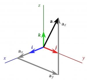
Those three vectors correspond, respectively, to the motion along the three axes.

It will often be convenient to use a shorthand for the time derivative, namely put a dot above the differentiated quantity. And so, for instance, one can write down the expression for the acceleration $\vec{a}$ , or the rate of change of the velocity, in a variety of equivalent ways:

(3) $\begin{equation*} \vec{a} \equiv \frac{d \vec{v}}{dt} \equiv \dot{\vec{v}} = \frac{d^2 \vec{r}}{dt^2} \equiv \ddot{\vec{r}} \end{equation*}$

Note that astronomers and navigators had been predicting the motion of celestial bodies for thousands of years before the development of Mechanics, using the regularities of empirical data on the motion of stars and planets. Their assumption was that the observed trends would continue in the future. The breakthrough brought by the modern science is that now we can often predict things in the future without reference to the prior history. Instead, we use laws of physics to write down and solve equations that require, as input, only the configuration of the system at the initial moment, not the prior history. In those cases when the knowledge of history is in fact needed, the equations tell us so. When we deal with very many particles, things can get complicated yet we can still make predictions about some average properties of the system, which is the formal essence of Thermodynamics.

The way I wish to review some basic notions of Mechanics here is decidedly modern and probably not the way Newton or Hooke would have done it.

Momentum: The most basic object in the theory is the momentum. The momentum $\vec{p}$ of a particle is defined as product of particle’s mass $m$ and velocity $\vec{v}$ :

(4) $\begin{equation*} \vec{p} = m \vec{v} \end{equation*}$

.

Whenever possible, we will usе 1D motion for mathematical illustrations, in which case one can get away without using the vector notation:

(5) $\begin{equation*} p = mv \end{equation*}$

with the understanding that the quantities $p$ and $v$ can be either positive or negative, the positive sign corresponding to rightward motion, the negative sign corresponding to leftward motion.

For a collection of particles, the total momentum is defined as the sum over the individual particles:

$\vec{P} = \sum_i \vec{p}_i$

.

The basic utility of the momentum comes from the empirical fact that the total momentum of a collection of particles, interacting or not, is conserved (i.e. remains fixed) in the absence of external forces. Furthermore, when a non-vanishing force is present, denote it with $f$ , then the momentum changes at the rate equal to the force itself:

(6) $\begin{equation*} \dot{\vec{p}} \equiv \frac{d \vec{p}}{dt} = \vec{f} \end{equation*}$

or

(7) $\begin{equation*} \dot{p} = f \end{equation*}$

in 1D. Eq. (6) (and Eq. (7)) is a mathematical statement of Newton’s 2nd law of Mechanics. In view of Eq. (4), Newton’s 2nd law can be also written explicitly as a differential equation for the velocity or the coordinate:

(8) $\begin{align*} m \dot{v} = f \\ m \ddot{x} = f \end{align*}$

The momentum may seem like a rather abstract notion. It is indeed. Yet it allows one to immediately rationalize some rather concrete phenomena of practical importance. Suppose you are floating leisurely in water next to a stationary object, such as a boat. Your mass is $m$ and the boat’s mass is $M$ . Imagine next you push yourself away from the boat. Because the total momentum of the you+boat system should remain constant and, hence, equal to its initial value of zero, it must be true that after you are done pushing, the ratio of the boat’s velocity to yours should be equal to $m/M$ . ( $0 = m v_\text{you} + M v_\text{boat} \Rightarrow v_\text{boat}/v_\text{you} = -m/M$ .) That is, the heavier the boat, the more slowly it will be moving at the end of the interaction. In other words, a heavier object exhibits more inertia. I’m sure you can come up with good examples from sports like football, basketball, wrestling, etc. As you may imagine, molecules will follow exactly the same trend when bouncing off one another.

In a great variety of important applications, the force depends on the coordinate of the particle. For instance, for a spring stretched or contracted by the amount $x$ off its equilibrium length:

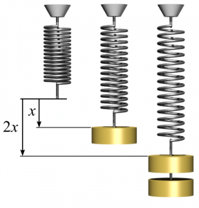
(Picture by Svjo – Own work, CC BY-SA 3.0, Link)

the restoring force is proportional to the displacement itself, i.e., the famous Hooke’s Law:

(9) $\begin{equation*} f = - k x \end{equation*}$

where the positive quantity $k$ is called the spring constant. When the force depends exclusively on the coordinate, it will be often very convenient to work not with the force itself but with a related function called the potential of the force, also referred to as the potential energy $V(x)$ . In 1D, the potential is defined as any function whose spatial derivative is equal to the force:

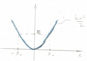
(10) $\begin{equation*} f\:=\:-\frac{dV}{dx} \begin{equation*} \end{equation*}$

And so, the potential corresponding to the restoring force of a spring from Eq. (9) is a simple parabola:

(11) $\begin{equation*} V(x) = \frac{k x^2}{2} \end{equation*}$

This simple parabolic potential is often called the harmonic potential, while the corresponding degree of freedom (the coordinate $x$ , in this case) is often referred to as the harmonic oscillator. The “oscillations” will be discussed later in this Chapter. It is instructive to sketch the potential energy (11). It is a parabola with positive curvature, much like a tea cup with its bottom down. It is easy to check, using Eq. (10) that the force to this potential is always restoring, i.e., it pushed the object toward the equilibrium point, where $f=0$ . A great advantage of working with potentials, as opposed to forces, is that this framework immediately appeals to our intuitive sense that things subjected to gravity tend to move to lower places. For low-magnitude vibrations, the harmonic potential from Eq. (11) is often a good approximation to other types of potentials, such as the typical potential of inter-molecular or inter-atomic forces:

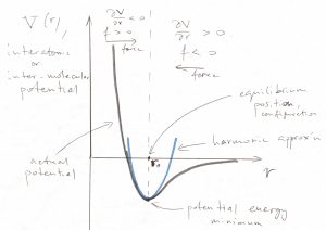
Though more complicated than the harmonic potential (11), this typical intermolecular potential still has a unique stable minimum. Generally, however, there are other types of equilibrium, where by equilibrium we mean a vanishing force, $f=0$ . In most cases of practical interest, this means the corresponding potential has a stationary point there: $dV/dx = 0$ , by Eq. (10).

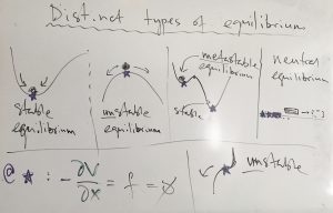
In the case of unstable equilibrium, there is no restoring force for a particle pushed off the maximum; on the contrary the emerged force will push the particle further away from the equilibrium point. When equilibrium is metastable, the system does exhibit a restoring force but only within a finite range of the coordinate. Neutral equilibrium means no force altogether, at any location. We will learn in this class that a variety of quantities, ranging from a bond length to the volume of a macroscopic system often can be thought of as degrees of freedom that are subject to a potential energy like those depicted above.

In spatial dimensions higher than one, instead of the relatively simple (10) one would have $f_x = -\partial V/ \partial x$ , $f_y = -\partial V/\partial y$ , etc. To avoid confusion, we note that in 1D, it is always possible to find a potential of the force for any force that depends exclusively on the coordinate, see Eq. (21) below, but this is not necessarily so in spatial dimensions 2 and higher. In any event, because the derivative of a constant vanishes, adding a constant to the potential does not modify the value of the force. If a force does allow for a potential, the force is called conservative, for reasons that will become clear shortly.

An important example of a reaction force that depends exclusively on the velocity is the force of friction such as that due to a viscous drag:

(12) $\begin{equation*} \vec{f}\:=\:-\zeta \: \vec{v}\ \end{equation*}$

where we have defined a new, positive quantity $\zeta$ , which is called the friction (or damping) coefficient. This friction force acts in the direction exactly opposite of the velocity.

Let us now introduce another, extremely important quantity called the kinetic energy. The kinetic energy for a single object is defined as follows:

(13) $\begin{equation*} E_\text{kin} \:=\: \frac{m v^2}{2} \end{equation*}$

For a collection of point masses, it is given by the expression

(14) $\begin{equation*} E_\text{kin}^\text{(total)} \:=\: \sum_j \frac{m_j v_j^2}{2} \end{equation*}$

This expression will resurface in due time as the energy of the ideal gas.

The kinetic energy—and any type of energy for that matter—is admittedly a very artificial concept. One might even say it is a contrived concept. Yet it is remarkably useful. Indeed, let’s consider the sum of the kinetic and potential energy, call it the energy:

(15) $\begin{equation*} E \:=\:\frac{m \: v^2}{2}\:+\:V(x) \end{equation*}$

Let us now compute the full time derivative of this quantity, using the chain rule of differentiation:

(16) $\begin{equation*} \frac{dE}{dt} \:=\: \frac{d}{dt} \: \left[ \frac{m \: v^2}{2}\:+\:V(x) \right] \:=\: m \: v \: \frac{dv}{dt}\:+\:\frac{dV}{dx} \:\frac{dx}{dt}\:=\: v \: \left(m \: \frac{dv}{dt} \:+\: \frac{dV}{dx} \right) \end{equation*}$

where we used that $dx/dt = v$ is the velocity, Eq. (2).

But, according to Newton’s second law, Eq. (8) and the relation (10),

(17) $\begin{equation*} m\: \:\frac{dv}{dt}\:=\:f\:=\:-\frac{\partial{V}}{\partial{x}} \end{equation*}$

Thus,

(18) $\begin{equation*} \dot{E} = 0 \:\: \Rightarrow \:\: E = \text{const} \end{equation*}$

Thus we obtain that if the motion of a body is subject to a conservative force, the energy of this body is conserved, that is, remains constant over time. This is the reason why forces of the type (10) are called conservative. Because of energy conservation, an increase in the potential energy should be accompanied by a decrease in the kinetic energy, the two exactly compensating each other.

In contrast with conservative forces, forces of the type (12) are dissipative, because they always cause the energy of the body to decrease, see below. The effect of inter-molecular collisions is often well approximated with such frictional forces. The energy is taken away from the body in question and passed on to those molecules that collide with the body. The total energy is however conserved.

As a consequence, the total energy of a collection of bodies that is isolated from the rest of the world remains constant over time. Conversely, if the energy of the system does happen to change, we know that an act of interaction with the environment must have occurred. This notion will come in handy later on when we discuss statistics of distinct microscopic configurations of various systems of interest.

FYI: Momentum and energy conservation are intrinsically related (which was revealed by Einstein’s theory of relativity) and can be interpreted as the invariance of physical laws with respect to space and time translation, respectively. (This is the gist of a famous theorem due to Emmy Noether, https://en.wikipedia.org/wiki/Emmy_Noether). In other words, the laws of physics are the same everywhere in space and do not change over time either.

The apparent conservation of momentum and energy is of great value in a number of ways. In addition to revealing deep properties of space and time, they often make it easier for us to solve problems of interest, as we have already seen in the boat example earlier.

Let us consider the energy of a particle subject to a conservative force, see Eq. (15) in which case the energy stays constant. Equating the energy values at two distinct times yields:

(19) $\begin{equation*} \frac{m\:v_1^2}{2}\:+\:V(x_1)\:=\:\frac{m\:v_2^2}{2}\:+\:V(x_2) \end{equation*}$

Thus one gets that the increment of the kinetic energy is the negative of the increment of the potential energy:

(20) $\begin{equation*} \Delta \frac{m v^2}{2} \: \equiv \: \frac{mv^2}{2} \Big|_1^2 \: \equiv \: \frac{m v_2^2}{2}\:-\:\frac{m v_1^2}{2} \:=\: -V(x_2)\:+\:V(x_1) \equiv -\Delta V(x) \end{equation*}$

In turn, the potential energy increment can be presented as the integral of the force, with the minus sign:

(21) $\begin{equation*} \Delta V(x) \equiv V(x_2)\:-\:V(x_1) = \int_1^2 dV(x) = \int_1^2 \frac{dV}{dx}\:dx\:=\: - \int_1^2f\:dx \end{equation*}$

Note that this equation represents the reciprocal operation to that in Eq. (10). The figure below graphically reviews the notion of the definite integral and two specific approximations used to compute such an integral:

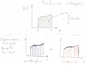
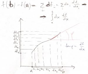
The second approximation, where we compute the total area of the shape by adding together the areas of the trapezoids, can be used to show rather explicitly that the increment of a function over a finite change in the argument is simply the integral of the derivative of that function:

Let us now introduce a new object, called the work of a force, the force can be conservative or non-conservative:

(22) $\begin{equation*} W_{1\to 2} = \int_1^2 f dx \end{equation*}$

The work is positive when the force $f$ and displacement $dx$ are in the same direction and negative otherwise. This is an intuitive notion: “If the force gets its way, the work is positive; if not, the work is negative”. For instance, when you lift an object, you perform positive work, while the force of gravity performs negative work.

According to Eq. (21), the work performed by a conservative force acting on an object is simply equal to the negative increment in the potential accompanying the displacement:

(23) $\begin{equation*} W_{1\to 2} \: = \: -\Delta V(x) \text{ , if the force is conservative:} f = -\frac{dV}{dx} \end{equation*}$

Note we could not make an analogous statement for non-conservative forces, for which one cannot even define a potential!

Eqs. (20) and (21) thus yield for the change in the kinetic energy of an object acted upon by conservative forces exclusively:

(24) $\begin{equation*} \Delta \frac{m v^2}{2} \:=\: -\Delta V(x) \:=\: W_{1\to 2} \end{equation*}$

Since the kinetic energy can be thought of as the intrinsic energy of the object proper (while the force represents an external agent) we arrive at the intuitive conclusion that

Positive work by external force → increase in internal energy
Negative work by external force → decrease in internal energy

Note the work of frictional forces is always negative: $-\zeta v \times dx = -\zeta (dx/dt) \times dx = -\zeta (dx)^2/dt < 0$ , since time increments are always positive. (This is why time travel is impossible.)

Some examples of practical applications of the law of conservation of energy

Our first example will be for the simple yet incredibly important case of a spatially uniform (i.e. “same everywhere”) force. This is a good approximation for the force of gravity for distances from the ground that are much smaller than the Earth’s size. A body of mass $m$ is subject to a force of gravity $-mg$ , where the minus sign indicates that the force is downward. (The coordinate axis we use to specify the displacement is oriented upward.) By Eq. (21), the potential difference between two points at height $x_2$ and $x_1$ respectively is, then, $V(x_2) - V(x_1) = m g \: (x_2-x_1)$ . Thus, for instance, an object that moves inertially uphill will be losing its kinetic energy as its height increases:

(25) $\begin{equation*} \frac{m\:v_2^2}{2}\:-\:\frac{m\:v_1^2}{2}\:=\:-mgh \end{equation*}$

This can be used to immediately deduce how high a projectile will high, if its vertical velocity is $v$ . Setting $v_2=0$ and $v_1=v$ in the equation above yields $h = v^2/2g$ . Analogously, an object dropped from height $h$ will reach the velocity $\sqrt{2 g h}$ just before it hits the ground. Note we didn’t have to solve any differential equations to obtain these estimates. Pretty convenient, isn’t it?

We can use these ideas to understand why solvated protein molecules do not sink to the bottom of the container even though protein mass density is about 1.2 g/cm³ , which is greater than that density of liquid water. The typical energy of an individual protein molecule is $k_B \:T$ (to be derived later) where the Boltzmann constant $k_B$ is numerically 1.38 x 10^-23 J/K and $T$ is temperature. 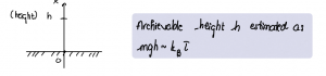This typical energy scale is to be compared with $mgh$ , where $h$ is the height of the flask. One can easily check that the variation of the potential energy, as a protein molecule traverses vertically the flask, are much smaller than the typical energy of the molecule: $mgh \ll k_B T$ . In other words, the potential energy variations in this case are only a tiny perturbation implying that the protein density variations due to the field of gravity would be small, too. Conversely, one can estimate the largest achievable height for a particle possessing a typical thermal energy, which, then, allows one to estimate the height of the atmosphere:

Now, even if energy conservation does not absolve us from having to solve a differential equation, it often helps to make it easier, which brings us to our second example, viz., 1D motion subject to a conservative force. Newton’s 2nd law implies the following 2nd order differential equation for the motion:

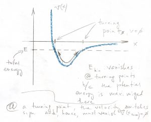
(26) $\begin{equation*} m \: \frac{d^2 x}{dt^2} = - \frac{dV}{dx} \end{equation*}$

which is generally hard to solve. Energy conservation allows one to reduce this problem to a 1st order differential equation. Indeed, the total energy is fixed and, furthermore, equal to the value of the potential energy at any of the turning points $x_\text{turning}$ . This is because at a turning point, the velocity switches sign and, thus, must vanish. As a result, the kinetic energy at turning points is zero (in 1D). Therefore,

(27) $\begin{equation*} \frac{mv^2}{2}\:+\: V(x) \:=\: \text{constant} \:=\: V(x_\text{turning}) \end{equation*}$

For the harmonic oscillator, this leads to:

(28) $\begin{equation*} \frac{dx}{\sqrt{x_0^2 - x^2}} = (2k/m)^{1/2} dt \end{equation*}$

because the turning points are $x_0$ and $(-x_0)$ .

The equation above is straightforwardly integrated using standard Tables of Integrals. For instance, if we choose the integration constant so that the particle is at the r.h.s. turning point at time zero, $x(t=0)=x_0$ , then one obtains:

(29) $\begin{equation*} x = x_0 \cos(\omega t) \end{equation*}$

where the quantity

(30) $\begin{equation*} \omega \equiv \sqrt{k/m} \end{equation*}$

is the oscillator’s circular frequency. (Can you use the just obtained solution for $x(t)$ to check that the total energy of harmonic oscillator is conserved?) Note the harmonic oscillator is a unique dynamical system in that its period of oscillation does not depend on the magnitude of the motion!

Two examples of combined applications of the laws of conservation of energy and of conservation of momentum

Two final examples involve collisions of objects, which will come in handy soon, when we discuss molecular scale processes.

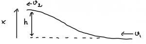
Imagine two moving objects that collide, stick together upon the collision, and then continue motion as a compound object:

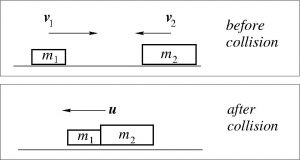
The collision leads to very complicated processes inside the bodies, such as shock waves, heating and what not, yet the fact of momentum conservation allows us to evaluate the velocity of the compound object without having to solve any equations:

$m_1\:v_1\:+\:m_2\:v_2\:=\:(m_1\:+\:m_2)\: u$

We can now evaluate the change in the kinetic energy:

(31) $\begin{equation*} \frac{(m_1+m_2) u^2}{2} - \left( \frac{m_1\:v_1^2}{2}\:+\:\frac{m_2\:v_2^2}{2} \right) = -\frac{(m_1\:m_2)(v_1\:-\:v_2)^2}{2(m_1\:+\:m_2)} \le 0 \end{equation*}$

The kinetic energy clearly decreases as a result of the collision, since in order for the two objects to collide, their velocity must be different. Where did the missing energy go? Since there are no external forces involved, this energy must have gone on to heat up the compound object! A collision where any amount energy has been dissipated into heat is called inelastic.

To finish, we will consider the opposite extreme limit of a purely elastic collision:

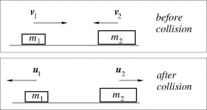
In this case, the momentum and energy conservation yield two equations:

$m_1\:v_1\:+\:m_2\:v_2\:=\:m_1\:u_1\:+\:m_2\:u_2$

$\frac{m_1\:v_1^2}{2}\:+\:\frac{m_2\:v_2^2}{2}\:=\:\frac{m_1\:u_1^2}{2}\:+\:\frac{m_2\:u_2^2}{2}$

which can be solved for two unknowns, namely, the velocities of the objects after the collision is over:

(32) $\begin{equation*} u_1\:=\:-v_1 \:+\:2 \frac{m_1\:v_1\:+\:m_2\:v_2}{m_1\:+\:m_2} \end{equation*}$

(33) $\begin{equation*} u_2\:=\:-v_2 \:+\:2 \frac{m_1\:v_1\:+\:m_2\:v_2}{m_1\:+\:m_2} \end{equation*}$

FYI: The above solution could have been obtained even in a simpler fashion by transferring to the reference frame moving with the center of mass, $v_\text{CM} = \frac{m_1\:v_1\:+\:m_2\:v_2}{m_1\:+\:m_2}$ , and then noting that in that frame, the position of the center of mass is immutable, as if it were an infinitely heavy wall. Since no energy is dissipated, each object will bounce off that “wall” with the velocity equal in magnitude to the incoming velocity, but opposite in sign. Transferring back to the original reference frame yields, then, Eqs. (32) and (33). Working in the reference frame moving with the center of mass also makes it clear that for collisions that are not completely elastic the particles will recoil less. Most dissipation occurs when the bodies don’t bounce at all, i.e., when they end up stuck together. This is exactly the situation we considered in the preceding example.

License

Icon for the Creative Commons Attribution-NonCommercial-NoDerivatives 4.0 International License

Basic Notions of Thermodynamics and Quantum Mechanics for Natural Sciences Copyright © 2020 by Vassiliy Lubchenko is licensed under a Creative Commons Attribution-NonCommercial-NoDerivatives 4.0 International License, except where otherwise noted.

License

Share This Book