Foundations of Quantum Mechanics. Operators. Wave function. The Schrodinger Equation.

Vassiliy Lubchenko

11 Foundations of Quantum Mechanics. Operators. Wave function. The Schrodinger Equation.

By the end of the 19th century, mathematical physicists became very good at solving Newton’s equations of motion for particles and the equations of motion for waves, such as light waves or sound waves, due to D’Alember, Euler, and others. So advanced was the state of mathematics that some proclaimed soon there would be no open physical questions to solve. Indeed, the physical models and much of the mathematics we still use to describe electromagnetic, gravitational, acoustic, and thermal phenomena, among others, were developed already in the 19th century. At the same time, experimenters were rapidly improving their methods, too, thus becoming able to study physical phenomena at progressively smaller length scales and shorter times scales. And that is when it became clear that something is missing in the classical description. Those open questions are too many to list here. We will limit ourselves to only a few. Some of these questions we will be able to address in a qualitative fashion.

Perhaps of most importance for Chemistry and Biology is the following question: How is it possible for bound states, such as atoms, molecules, or solids to exist? Electrons are known to be negatively charged and atomic nuclei to be positively charged. According to Earnshaw’s Theorem (1842), a set of electrical charges is unstable. Yet somehow electrons manage to stick around atomic nuclei, seemingly forever, without falling on the nuclei. The resulting finite size of atoms underlies the very notion of a particle and the notion of matter itself. Furthermore, if one takes the classical perspective that electrons spin around the nucleus, they must emit radiation because their motion is constantly accelerating toward the nucleus, because of the Coulomb attraction between the two charges. Indeed, the only way for an accelerating/decelerating charge to exchange the energy with the rest of the world is to emit/absorb radiation; this is how radio transmitters and synchrotrons actually work. Following this continuous loss of energy, the electrons must eventually fall on the nucleus. Yet they do not, nor is there any radiation emitted by atoms or molecules in their lowest-energy state. (Note bodies that spin around each other owing to the mutual gravitational pull do emit gravity waves, which eventually leads to their collision.)
Classical Physics implies that the energy of an electron spinning around a nucleus can take arbitrary (negative) values, yet the absorption spectra of gases indicate that the energy of the electron changes in discrete bits. For instance, the energy of a hydrogen atom can have any of the following values: $E_n = -\text{const}/n^2$ , where $n=0, 1, 2, \ldots$ . In addition to its basic significance, this notion underlies the field of spectroscopy, which is arguably the most important experimental tool of natural sciences.
Classical Physics does not offer a way to approach the fundamental question of whether there is a smallest indivisible unit of matter, thus creating a difficult conceptual problem.
Why are there seemingly two, seeming distinct ways for energy to travel through space, that is, in terms of compact particles and in terms of waves? Furthermore, these two distinct ways are actually not mutually exclusive for massive particles, and is made clear from the interference patterns created by electronic beams. https://en.wikipedia.org/wiki/Electron_diffraction
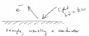
One of the worst problems for Classical Physics is the photoelectric effect. Hereby, a solid exposed to light with a wavelength shorter than a certain threshold value emits electrons. Surprisingly, the energy of an individual electron does not increase with the light’s intensity, but depends only on the light’s frequency $\nu$ , according to the following formula:
(1) $\begin{equation*} E_\text{electron} \:=\: h \nu - W \end{equation*}$

The quantity $W$ is called the work function. No electrons are emitted for $\nu < W/h$ . Classically, nothing prevents a material from ejecting an electron once some requisite amount of energy is absorbed. The energy can be delivered using light of any frequency, including those less than $W/\nu$ , subject to the intensity and exposure time, of course. Nor is there a constraint on the relation between the energy of the ejected electron and the light’s frequency. In contradistinction with these expectations, there seems to be a smallest amount—or “quantum”—of energy that can be absorbed by the sample per absorption event. (In practice, photoelectric spectroscopy is usually done on conducting samples so that the negative charge can be replenished. Non-conductive samples quickly become positively charged which increases the work function over time.) In fact, this quantum of energy is equal to $h \nu$ , while the work function $W$ , then, represents the smallest value of the binding energy of the electron in the solid.

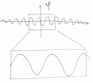
Quantum Mechanics has successfully resolved those and many more issues; it is regarded as one of the most successful microscopic descriptions. From the mathematical perspective, the main object of this description is the wave packet, which is a function of both space and time. At a specific value of time, it is a function of the coordinate only, as we show below:

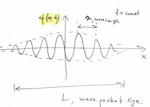
We see that the notion of a wave packet combines the notions of a wave and a particle: The spatial extent $L$ of the packet can be regarded as the particle size. Indeed, so long as the spatial resolution of our experiment is greater than $L$ , the internal, “wavy” structure of the packet won’t even be detected. On the other hand, the oscillations within the packet can be regarded as wave-like, oscillatory motions and would be detectable given sufficient spatial resolution. Because at any given moment in time, a wave-packet is a function of the coordinate, call it $\psi(x)$ , it technically corresponds to an infinite number of degrees of freedom, one per each space-point $x$ . This drastically complicates the mathematics of the theory. In comparison, to describe the state of motion of a solid object in 3D, we only need to specify the location of its center of mass, its orientation, and the velocities of its translational and rotational motion, which, in total, is 12 variable at most.

If the wave packet moves in space as some non-zero speed, its locality in space also implies a locality in time:

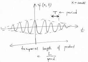
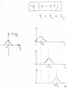
We, then, interpret the non-zero portion of the time dependence of the signal as the moment where our “particle-wave” passes through the point $x$ . From now on, we focus on wave packets in 1D that move to the right or the left without changing their shape. While not too constraining for our purposes here, this simplifies the algebra since now the coordinate and time enter our wave packet in a particular combination:

(2) $\begin{equation*} \psi(x, t) \:=\: f(x-vt) \end{equation*}$

where $f$ is some function. The figure below illustrates the time evolution of the packet, where we used a bell-shaped function $f$ for clarity. (Such rudimentary wave packets are allowed, but are hardly waves in the regular sense of the word.):

To develop a mathematical description for wave packets, we first “zoom in” on the central portion, which looks like a plane wave:

Let us for now focus exclusively on plane waves: Consider a cosine profile with an arbitrary amplitude $A$ and phase shift $\varphi_0$ :

(3) $\begin{eqnarray*}f(y) &=& A \, \cos \left(\frac{2\pi}{\lambda} y + \varphi_0 \right) \\ &=& A \, \left[ \cos \left(\frac{2\pi}{\lambda} y \right) \cos(\varphi_0) - \sin \left(\frac{2\pi}{\lambda} y \right) \sin(\varphi_0) \right] \\ &\equiv& C_1 \cos \left(\frac{2\pi}{\lambda} y \right) + C_2 \sin \left(\frac{2\pi}{\lambda} y \right) \end{eqnarray*}$

where $C_1 \equiv A_1 \cos(\phi_0)$ , $C_2 \equiv -A_1 \sin(\phi_0)$ , and we used the trigonometric formula $\cos(x+y)=\cos(x)\cos(y)-\sin(x)\sin(y)$ to derive the last equality. The latter equality demonstrates that any linear combination of $\cos$ and $\sin$ waves with the same period can be presented as a cosine wave with a phase shift. (It can be presented as a sine wave, as well, of course.) Note the denominator $\lambda$ was needed so that the argument of the cosine is dimensionless, while the factor $2 \pi$ is introduced simply for convenience so that the function is periodic with period $\lambda$ . (Recall that the functions $\cos x$ and $\sin x$ are periodic with period $2 \pi$ .) The quantity $\lambda$ is called the wavelength, which it really is. It is convenient to introduce a new quantity called the wave vector:

(4) $\begin{equation*} k\: \equiv \: \frac{2\pi}{\lambda} \end{equation*}$

The resulting plane wave is, then,

(5) $\begin{equation*} \psi_\text{mc}(x, t) \:=\: A \, \cos [k (x-vt) + \varphi_0] \:\equiv \: C_1 \cos (k x- \omega t) \:+\: C_2 \sin (k x- \omega t) \end{equation*}$

where we used a trigonometric identity $\cos(a+b)=\cos (a) \cos(b) - \sin (a) \sin(b)$ and have introduced yet another quantity, called the circular (or angular, or cyclic) frequency:

(6) $\begin{equation*} \omega \: \equiv \: k \, v \: =\: 2 \pi \frac{v}{\lambda} \: =\: \frac{2 \pi}{T} \: =\: 2 \pi \, \nu \end{equation*}$

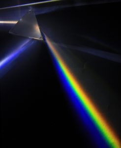
since the wavelength is the distance traveled by the wave in one period of the oscillation, $\lambda=v T$ ,while the regular frequency, $\nu=1/T$ , is simply the number of oscillations per unit time; there is exactly one oscillation per period of the wave.We used the subscript “mc” in Eq. 5 to signify “mono-chromatic”, since our signal is characterized by a single oscillation frequency. There is one-to-one correspondence between the frequency of light waves and their color (Image: D-Kuru, CC BY-SA 3.0 AT, via Wikimedia Commons):

The circular frequency $\omega$ is more convenient than the standard frequency $\nu$ because we don’t have to drag along the $2\pi$ factor, and so we shall use exclusively $\omega$ , not $\nu$ , while calling it simply the frequency. In this notation, the energy of a light quantum becomes:

(7) $\begin{equation*} h \, \nu \:=\: \frac{h}{2 \pi} \: 2 \pi \, \nu \: \equiv \: \hbar \, \omega \end{equation*}$

where $\hbar$ (pronounced ‘h-bar’) is a version of Planck’s constant:

(8) $\begin{equation*} \hbar \: \approx \: 1.05 \cdot 10^{-34} \text{J sec}\end{equation*}$

Though used frequently for practical applications, the constant $\hbar$ is of no fundamental significance; it is simply a means of inter-converting between frequency and energy scales, similarly to how the Boltzmann constant is a means of inter-converting between Joules and Kelvins. This said, the central notion of the correspondence between frequency and energy:

(9) $\begin{equation*} E \:=\: \hbar \, \omega \end{equation*}$

is not at all obvious, although it is natural for many reasons some of which will become clearer in due time. Here we take the correspondence between the frequency of a cyclic motion and its energy—which is at the very heart of Quantum Mechanics—as an experimental fact implied by the photoelectric effect.

Our next task to establish how we can describe the dynamics of inertial objects using operations that can be applied to waves. (This is a non-trivial task because excitations that we know are wave-like, such as light or sound, are actually massless!) Specifically, we know that the energy $E$ of an inertial object is given the expression

(10) $\begin{equation*} E \:=\: \frac{p^2}{2m} \:+\: V(x) \end{equation*}$

where $p$ is the momentum. The potential energy $V(x)$ is something that is there irrespective of whether the wavepacket is present or not. Thus we only need to determine a mathematical operation to extract the energy and momentum from the functional form of a wave packet.

First we tackle the total energy and take advantage of the simple linear connection 9 between the frequency and energy. What is the mathematical operation that would allow us to extract the frequency $\omega$ ? We notice that for the monochromatic wave signal from Eq. 5, differentiating twice w.r.t. to time produces the same wave signal, but multiplied by $(-\omega^2)$ :

(11) $\begin{equation*} \frac{\partial^2}{\partial t^2 } \psi_\text{mc}\:=\:-{\omega}^2 A \, \cos [k (x-vt) + \varphi_0] \:=\:-{\omega}^2 \psi_\text{mc} \end{equation*}$

Thus we establish that there is, in fact, a mathematical operation that extracts the frequency squared:

(12) $\begin{equation*} -\frac{\frac{\partial^2}{\partial t^2 } \psi_\text{mc}}{\psi_\text{mc}} \:=\: \omega^2 \end{equation*}$

Mathematical situations exemplified by Eq. 11, where an application of a mathematical operation— or operator—to a function produces the very same function times a fixed number are of significance to us. Generally, we say that if some operator $\hat{O}$ , when applied to a function, produces the very same function times a fixed number:

(13) $\begin{equation*} \hat{O} \, f \:=\: \lambda \, f \end{equation*}$

we call the function $f$ an eigenfunction of the operator $\hat{O}$ , where the number $\lambda$ is the corresponding eigenvalue.

Arguably the simplest operator is when one simply multiplies a function by a constant:

(14) $\begin{equation*} \hat{O} \: \equiv \: C \end{equation*}$

Since $C \, f(x) = C \, f(x)$ for any function $f$ , this means that every function is a eigenfunction of the multiplication operator, where the multiplier itself is the corresponding eigenvalue. A less trivial example is the operation of differentiation:

(15) $\begin{equation*} \hat{O} \:\equiv\: \frac{\partial }{\partial x} \end{equation*}$

To determine the eigenfunction, if any, of this operator we must solve a differential equation, as seen by substituting the above equation into Eq. 13:

(16) $\begin{equation*} \frac{\partial }{\partial x} f \:=\: \lambda \, f \end{equation*}$

This is, of course, a very familiar differential equation that is solved by the exponential function

(17) $\begin{equation*} f(x) \:=\: A \, e^{\lambda \, x} \end{equation*}$

where $A$ is an arbitrary constant. This is a general pattern for linear operators:

(18) $\begin{equation*} \hat{O} \, A \, f \:=\: A\, \hat{O} \, f \end{equation*}$

If a function is an eigenfunction of a linear operator, then multiplying this function by an arbitrary constant also produces an eigenfunction. This embarrassment of riches, so to speak, is never a problem, since we usually end up normalizing our eigenfunction as appropritate to the task at hand. This does bring about an important point that we are generally interested in eigenfuctions that are normalizable, to be discussed in more detail a bit later. In the rest of the class, we will focus exclusively on linear operators.

To give one more example of a linear operator, consider this:

(19) $\begin{equation*} \hat{O} \:\equiv\: x \, \frac{\partial }{\partial x} \end{equation*}$

It is not difficult to see that this operator has the power law function as its eigenfunction

(20) $\begin{equation*} f(x) \:=\: A x^n \end{equation*}$

where $n$ is the corresponding eigenvalue and $A$ is an arbitrary constant. This is because $x \frac{d}{dx} A x^n = A \: x \: n x^{n-1} = n \, A x^n$ .

Let us return to the search for a linear operator that would extract $\omega$ . Simply taking a square root from Eq. 12 won’t do us much good since the operation $\sqrt{\hat{O} f}$ produces a quantity going as $f^{1/2}$ , which is generally not equal to $f$ times a constant. One might think that differentiation once w.r.t. $t$ would do the trick since it brings down a factor of $\omega$ , but, according to Eqs. 15 through 17, the corresponding eigenfunction would be an exponential function $e^{\omega \, t}$ , not on oscillatory function we need to describe a wave. Undeterred, we go ahead and apply the $\frac{\partial}{\partial t}$ operator to the function 5

(21) $\begin{equation*} \frac{\partial}{\partial t} [ C_1 \cos (k x- \omega t) \:+\: C_2 \sin (k x- \omega t) ] \:=\: \omega C_1 \sin (k x- \omega t) \:-\: \omega C_2 \cos (k x- \omega t) \end{equation*}$

and ask whether this can be made equal to $\lambda [ C_1 \cos (k x- \omega t) \:+\: C_2 \sin (k x- \omega t) ]$ , where $\lambda$ , then, would be the eigenvalue. Equating this to the r.h.s. of Eq.21 yields

(22) $\begin{align*} &\lambda C_1 \:=\: \omega C_2 \\ &\lambda C_2 \:=\: -\omega C_1 \end{align*}$

This system of equations has an infinite number of solutions. After dividing the top equation by the bottom equation, one observes that for each of those solutions, however, it must be true that

(23) $\begin{equation*} C_1^2 \:=\: -C_2^2 \end{equation*}$

This implies that one of the numbers $C_1$ and $C_2$ must be the square root of a negative number! Although disconcerting at first, this seemingly absurd idea shouldn’t be discarded quite yet. To give an historical example, the ancients couldn’t accept for the longest time the concept of a negative number, and whenever negative numbers appeared in calculations as intermediate results they simply thought of those as being “owed”. For instance the operation $2+3$ makes perfect sense, but the equivalent operation $2 + 3=2+(8-5)=2-5+8=-3 + 8$ involves a negative number as an intermediate result. One may think of this $-3$ number as a result of owing somebody 3 dollars while physically having 8 dollars on hand, and so the effective total is still positive and everything is fine. For instance, suppose you have $1,000, which you can spend as you please, but, at the same time, you owe your bank $1,500. In effect, you total assets are actually negative: -$500. Yet both you and the bank have positive amounts of money, and so there is no need to use negative numbers so long as we are willing to use the concept of debt. Yet for the efficiency of mathematical computation, it is easier to simply use negative numbers.

By the same token, let us generalize the concept of multiplication by allowing the square of a number to be negative in an intermediate calculation, so long as the final result does not involve such “aberrant” numbers. For concreteness, we set

(24) $\begin{align*} C_1 \:=\: 1 \\ C_2 \:=\: i \end{align*}$

where we define a new quantity $i$ , called the “imaginary” unit:

(25) $\begin{equation*} i^2 \:=\: -1 \end{equation*}$

So long as our final answer does not involve $i$ , we should regard it simply as a convenient computational tool, no more no less. Again, on a historical note, the imaginary unit appeared as an intermediate result already centuries ago, during ancient calculations of the roots of polynomial equations, sometimes even when the roots themselves were “normal” numbers whose squares were non-negative.

Thus we obtain

(26) $\begin{eqnarray*} \frac{\partial}{\partial t} [ \cos (k x- \omega t) \:+\: i \, \sin (k x- \omega t) ] &=& \omega \sin (k x- \omega t) \:-\: i \, \omega \cos (k x- \omega t) \\ &=& -i \omega [\cos(k x- \omega t) \:+\: i \sin (k x- \omega t)] \end{eqnarray*}$

i.e. the function $\cos (k x- \omega t) \:+\: i \, \sin (k x- \omega t)$ is an eigenfunction of the operator $\frac{\partial}{\partial t}$ with the corresponding eigenvalue $(-i \omega)$ . Likewise, one can show that

(27) $\begin{equation*} \frac{\partial}{\partial x} (\cos x \:+\: i \, \sin x) \:=\: i (\cos x \:+\: i \sin x) \end{equation*}$

Comparing this with Eqs. 15—17 shows that

(28) $\begin{equation*} e^{ix} = \cos x + i \sin x \end{equation*}$

which is the celebrated Euler’s formula. Expanding the exponential in the left hand side in the Taylor series yields

(29) $\begin{eqnarray*} e^{ix} = \sum_{n=0}^\infty \frac{(i)^n x^n}{n!} &=& \sum_{n=0}^\infty \frac{(i)^{2n} x^{2n}}{(2n)!}+ \sum_{n=0}^\infty \frac{(i)^{2n+1} x^{2n+1}}{(2n+1)!} \\ &=& \sum_{n=0}^\infty \frac{(-1)^{n} x^{2n}}{(2n)!}+ i \sum_{n=0}^\infty \frac{(-1)^{n} x^{2n+1}}{(2n+1)!} \end{eqnarray*}$

where we broke up the original sum into the sums over the even and odd powers of $x$ and used that $i^{2n} = (i^2)^n = (-1)^n$ . We recognize the two sums on the r.h.s. as the Taylor expansions for the cosine and sine functions, respectively, consistent with the Euler formula. (Neither of these two expansions contains the imaginary unit!) Hence, the imaginary unit $i$ is simply a clever bookkeeping device that allows us to simultaneously work with two numbers at a time. Such “compound” numbers, each of which is simply a pair of actual numbers, say $x$ and $y$ , are called complex numbers and are written as this

(30) $\begin{equation*} z \:=\:x \:+\:i \, y \:= \:i \, y \:+\: x\end{equation*}$

where $x$ is called the real part and $y$ is called the imaginary part, for historical reasons. The two numbers $x$ and $y$ are equally important, and there is nothing more real about the $x$ than the $y$ .

Now, for two complex numbers $z_1=x_1+i y_1$ and $z_2=x_2+i y_2$ ,

(31) $\begin{equation*} z_1\:+\:z_2\:=\:(x_1\:+\:x_2)\:+\:i(y_1\:+\:y_2) \end{equation*}$

where we observe that one can add two pairs of number in one shot by using complex numbers. A more interesting example is that where multiply two complex numbers:

(32) $\begin{eqnarray*} z_1 z_2 &=& (x_1\:+\:i y_1) (x_2\:+\:i y_2)\:=\:x_1 x_2\:+\:i^2 y_1 y_2\:+\:i(x_1y_2\:+\:x_2y_1) \\ &=& x_1 x_2\:-\: y_1 y_2\:+\:i(x_1y_2\:+\:x_2y_1) \end{eqnarray*}$

If we further substitute $x_1=x_2=x$ and $y_1=-y_2=y$ into the above equation, we obtain

(33) $\begin{equation*} z^* z \:=\: x^2 + y^2 \end{equation*}$

where we have introduced the complex conjugate of the number $z=x+iy$ :

(34) $\begin{equation*} z^* \:=\: x \:-\: i \, y\end{equation*}$

The complex number $z$ and its complex conjugate $z^*$ , when pictured on the $(x, y)$ plane, are mirror images of the other w.r.t. to the horizontal axis:

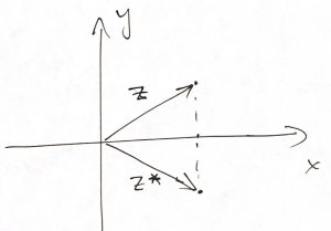
Because $x^2 + y^2$ is the length square of the vector whose endpoint is the location of the complex number $z$ , one customarily uses the following notation:

(35) $\begin{equation*} z^* z \: \equiv \: |z|^2 \end{equation*}$

Now, according to Eq. 26, the eigenvalue of the operator $\frac{\partial }{\partial t}$ is $-i \omega$ . Since $i \hbar \times (-i \omega) = \hbar \omega$ , we conclude the energy operator is given by:

(36) $\begin{equation*} \hat{H} \:=\: i\hbar \frac{\partial}{\partial{t}} \end{equation*}$

To extract the momentum of a wave, we use Einstein’s result on the connection between the energy and momentum that applies for both massive and mass-less objects:

(37) $\begin{equation*} E^2\:=\:p^2c^2\:+\:(m_0 c^2)^2 \end{equation*}$

where $p$ is the momentum, $c$ is the speed of light, and $m_0$ is the rest mass, i.e., the mass in the frame moving with the object. For a mass-less object, such as a particle of light, $m_0=0$ , and so

(38) $\begin{equation*} E\:=\:pc \end{equation*}$

while $E=\hbar \omega$ . Thus,

(39) $\begin{equation*} p \:=\: \hbar \frac{\omega}{c} \:=\: \hbar \, \frac{2\pi \nu}{c} \:=\: \hbar \, \frac{2\pi}{\lambda} \:=\: \hbar \, {k} \end{equation*}$

where $k\:=\:\frac{2\pi}{\lambda}$ is our old friend the wave vector.

Since

(40) $\begin{equation*} \frac{\partial}{\partial{x}} e^{i(kx-\omega{t})}\:=\: i \, k \,e^{i(kx-\omega{t})}\end{equation*}$

we conclude that the momentum operator is simply the derivative w.r.t. to the coordinate times $(-i \hbar)$ :

(41) $\begin{equation*} \hat{p}\:=\:-i\hbar\frac{\partial}{\partial{x}}\end{equation*}$

The kinetic energy operator, then, is given by

(42) $\begin{equation*} \frac{\hat{p}^2}{2 m } \:=\: \frac{1}{2m} \left(-i \hbar \, \frac{\partial}{\partial x}\right) \left(-i \hbar \, \frac{\partial}{\partial x}\right) \:=\: -\frac{\hbar^2}{2m} \frac{\partial^2}{\partial x^2} \end{equation*}$

Now we take the classical expression for the total energy $E\:=\:\frac{p^2}{2m}\:+\:V(x)$ and plug in it the quantum-mechanical values for $E$ and $p$ :

(43) $\begin{equation*} \frac{i\hbar \frac{\partial}{\partial{t}}\psi}{\psi }\:=\: \frac{ -\frac{{\hbar}^2}{2m}\frac{{\partial}^2}{\partial{x^2}}\psi}{\psi} \:+\: V(x) \end{equation*}$

After multiplying through by $\psi$ we obtain the celebrated Schrodinger Equation:

(44) $\begin{equation*} i\hbar\frac{\partial}{\partial{t}} \psi(x, t) \:=\: -\frac{{\hbar}^2}{2m}\frac{{\partial}^2}{\partial{x^2}}\psi(x, t) \:+\:V(x)\psi(x, t) \end{equation*}$

where we have explicitly indicated that the function $\psi(x,t)$ , which solves this equation, depends both on the time and coordinate. Accordingly, the above equation is sometimes called the time-dependent Schrodinger equation. Any solution of a Schrodinger equation are usually called a wave-function, for historical reasons.

Time dependent equations such as Eq. 44 are hard to solve. Fortunately, we are mostly interested here in solutions corresponding to bound states, which are stationary, i.e., time independent. To see how such solutions arise, we substitute the following functional for form in Eq. 43

(45) $\begin{equation*} \psi(x,\:t)\:=\:X(x) \, T(t) \end{equation*}$

i.e., we have presented the full wave-function as a product of a function that depends exclusively on the coordinate and a function that depends exclusively on time. This method of solving differential equations for functions of more than one variable is called “separation of variables”. We thus obtain

(46) $\begin{equation*} \frac{i\hbar \frac{\partial}{\partial{t}}\cdot{T(t)}}{T(t)}\:=\: \frac{[-\frac{{\hbar}^2}{2m}\frac{{\partial}^2}{\partial{x^2}}\:+\:V(x)]\cdot{X(x)}}{X(x)}\end{equation*}$

We observe that the l.h.s. depends exclusively depends on time, while the r.h.s. exclusively depends on the coordinate. But the time and coordinate are independent quantities, and so the above equation is meaningful when both sides are constants that are independent of $x$ and $t$ :

(47) $\begin{equation*} \frac{i\hbar \frac{\partial}{\partial{t}} {T(t)}}{T(t)} \:=\: \text{const} \end{equation*}$

(48) $\begin{equation*} \frac{[-\frac{{\hbar}^2}{2m}\frac{{\partial}^2}{\partial{x^2}}\:+\:V(x)]\cdot{X(x)}}{X(x)} \:=\: \text{const} \end{equation*}$

where the constant is the same in both equations. We now re-write Eq. 49 this way

(49) $\begin{equation*} i \hbar \frac{\partial}{\partial{t}}\cdot{T(t)} \:=\: \text{const} \: T(t) \end{equation*}$

while remembering that the operator on the l.h.s. is the energy operator. Thus the time dependent part of the variable-separated solution from Eq. 45 is an eigen-function of the energy operator, whose eigenvalue is, of course, the energy itself and is, by construction, a time-independent quantity:

(50) $\begin{equation*} \text{const} \:=\: E \end{equation*}$

Thus those variable-separated solutions are, in fact, energy conserving solutions. The value $E$ itself of the total energy is of yet unknown, unfortunately. The above equation can be however substituted into Eq. 48 to obtain the following equation:

(51) $\begin{equation*} \left[ - \frac{\hbar^2}{2m} \frac{d^2}{dx^2}\:+\:V(x) \right] {X(x)}\:=\:E \, X(x) \end{equation*}$

which is called the time-independent Schrodinger Equation, or, often, simply the Schrodinger Equation. Note we have replaced the partial derivative w.r.t. $x$ by the full derivative because the function $X$ depends only on $x$ .

Thus we observe that the task of determining the possible values of the energy of our system reduces to finding all possible eigenfunctions and eigenvalues of the operator on the left. This operator:

(52) $\begin{equation*} \hat{H}\:=\:-\frac{{\hbar}^2}{2m}\frac{{\partial}^2}{\partial{x^2}}\:+\:V(x) \end{equation*}$

is called the Hamiltonian operator. It depends exclusively on the coordinate and not on time. For each eigenvalue so found, one can immediately solve for the time-dependent part since now the constant in Eq. 49 is known:

(53) $\begin{equation*} i\hbar \frac{\partial}{\partial{t}} {T(t)} \:=\: E \, T(t) \: \Rightarrow \: T(t) \:=\: C e^{-iET/\hbar} \end{equation*}$

where $C$ is a constant. If we are fortunate enough to be able to determine all possible eigenfunctions and corresponding eigenvalues, then the solution to the full, time-dependent problem from Eq. 44 is a linear combination of those solutions:

(54) $\begin{eqnarray*} \psi(x, t) &=& \sum_j \, T_j(t) X_j(x) \\ &=& \sum_j \, C_j \, e^{-\frac{i E_j t}{\hbar}} \psi_j (x) \end{eqnarray*}$

where we use the label $j$ to denote distinct eigenfunctions. The above formula utilizes the notion that if each of two distinct functions solves a linear equation—Eq. 44 in this case—then their sum does, too.

The distinct eigenfunctions in Eq. 54 correspond to the distinct microstates we have already alluded to many times in the Thermo part of the Course. Now we have a way to actually determine those microstates, at least in principle. The corresponding eigevalues, $E_j$ , may or may not be numerically different. If the energy eigevalues for two or more distinct microstates happen to be numerically equal, we refer to that situation as the corresponding energy value being degenerate. As we have seen in the Thermo part, one expects that the degeneracy generally grows with $E$ . Since, $e^{-\frac{i E_j t}{\hbar}}=1$ in the beginning, $t=0$ , the constants $C_j$ must be chosen so that $\psi(x, t=0)$ matches the initial conditions of interest. For instance, imagine plucking a guitar string like on the l.h.s. below:

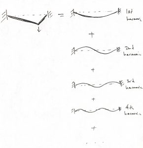
The r.h.s. of the picture exemplifies the eigenfunctions of the time-independent Schrodinger equation, where the energy eigenvalue increases from top to bottom. We observe that the initial spatial profile of the string resembles the lowest energy wavefunction quite a bit, but other harmonics must be admixed, with some weight, to fully recover that initial spatial profile. Because of this, the overall dynamics of the string will include motions at more than one energy and, hence, frequency. These high frequency motions can actually be heard when a musical instrument is played and are called “harmonics.” Similarly, we will sometimes informally refer to distinct solutions of the time-independent Schrodinger equation as harmonics. The general trend is that higher-order, shorter-wavelength harmonics correspond to higher energy motions. For a string, such higher frequency, higher energy motions mean a higher pitch sound.

Finally, to determine the meaning of the wave function itself, we again use insight from wave mechanics. There we know that the energy density of a wave is proportional to the wave’s amplitude squared. To interpret this from a particulate viewpoint, the energy density is equal to the energy per particle times the particle density. Thus the amplitude-squared is proportional to the particle density. Because our wave function generally consist of two contributions, corresponding to the real and imaginary parts of the wave function, we simply add together the contributions of the two parts. According to Eqs. 33 and 35 the density $p(x)$ of the particles at point $x$ is given by the quantity

(55) $\begin{equation*} p(x) \:=\: \psi^*(x,t) \psi(x,t) \:=\: |\psi(x,t)|^2 \:=\: |\psi^*(x,t)|^2 \end{equation*}$

The vast majority of textbooks postulates that $p(x)$ is the probability to find the particle(s) at location $x$ . While practical, this interpretation is misleading. That a quantity is distributed—and $p(x)$ certainly varies in space and time, in most cases—does not necessarily mean that the quantity is random. For instance, the digits of the number $\pi=3.141529\ldots$ may seem to be random–and are, in fact, uniformly distributed!—they are not at all random, but are computed using a specific procedure. Likewise, there is nothing stochastic about the quantum-mechanical equations of motion. (Though they are mightily complicated at times!) An interesting, somewhat advanced discussion of the probabilistic interpretations of Quantum Mechanics can be found at https://getpocket.com/explore/item/how-to-make-sense-of-quantum-physics?utm_source=pocket-newtab. Still, in most cases, we cannot fully control the initial conditions in experiment, and so the notion of $p(x)$ being a distribution of probability becomes quite accurate. As with any distribution, the chances of recovering values of $x$ within an interval $[x_1, x_2]$ are evaluated by integrating the distribution:

(56) $\begin{equation*} (\text{probability of } x_1 < x < x_2) \:=\: \int_{x_1}^{x_2} p(x) \, dx \:=\: \int_{x_1}^{x_2} |\psi(x,t)|^2 \, dx \end{equation*}$

In many cases, we are interested in one particle at a time, in which case the total probability to find the particle somewhere in space is 1. In such cases, we normalize the wavefunction to unity:

(57) $\begin{equation*} \int_{-\infty}^{\infty} |\psi(x,t)|^2 \, dx \:=\: 1\end{equation*}$

Having been primed by classical-physics training, many people struggle with the precise meaning of the quantum mechanical equations of motion and the wavefunction itself. This may explain continuing efforts to interpret quantum mechanics via purely classical means. Some of these of efforts are misguided, but some have resulted in useful ideas. For instance, Eq. 39 suggests that one may associate a wave length to a anything that has a momentum, such as a body moving with some speed $v$ and, hence, possessing momentum $p=mv$ . One may formally associate the following quantity of dimensions length to this motion, called the de Broglie wavelength:

(58) $\begin{equation*} \lambda_\text{dB} \:=\: \frac{2 \pi}{k} \:=\: \frac{2 \pi \hbar}{p} \:=\: \frac{2 \pi \hbar}{mv} \end{equation*}$

This yields an informal criterion for the motion of the object of size $L$ being classical:

(59) $\begin{equation*} \lambda_\text{dB} \:\ll\: L \end{equation*}$

A simple estimate shows that the de Broglie wavelength of a macroscopic object becomes incredibly small even at very very slow speeds. Note that such speeds cannot be any less than their thermal value, i.e., $v_\text{th} \sim (k_B T/m)^{1/2}$ . By convention we define the thermal de Broglie wave

(60) $\begin{equation*} \lambda_\text{dB, th} \:=\: \left( \frac{2 \pi \hbar^2}{m k_B T} \right)^{1/2}\end{equation*}$

which is simply the expression 58 for the regular de Broglie wavelength with the thermal velocity plugged in, times a constant of order one. Whenever the thermal de Broglie wavelength becomes comparable or greater than the particle size, we can expect quantum effects. For instance, the motions of protons in water are quite quantum-mechanical, which explains the unusually high dielectric susceptibility of water, among other things. For heavier atoms, quantum effects becomes less pronounced. In contrast, the motions of electrons are largely quantum mechanical, which is exceptionally important for bonding as we discuss in the next Chapter.

Bonus discussion: The normalization condition embodied in Eq. 57 partially fixes an aforementioned issue that each operator has an infinite number of equivalent eigenfunctions that differ only by an overall multiplicative number. The fix is not complete since the above equation only fixes the absolute value of the multiplicative constant, which could be either positive or negative or, generally, complex-valued. Remarkably, the seeming mathematical ambiguity has physical consequences, which we won’t have a chance to discuss in this Course except for one example, see the next Chapter. In any event, this ambiguity does not arise, if we confine ourselves to considering just one microstate at a time and the wavefunction of the microstate in question has a limited spatial extent. In such cases, one can use ideas from Linear Algebra to show that the solution of the time-independent Schrodinger equation 51 can always to be chosen to be real-valued, i.e., have just one, not the two components that were necessary to define a wave packet. This means, among other things, that every wave packet is wavefunction, but not every wavefunction is a wave-packet. Specifically, wave functions of bound states are not wavepackets. In physical terms, this is because bound states do not correspond to transfer of mass—and energy, momentum, etc.—through space, while wavepackets do transport energy through space. It is quite reasonable, and even beneficial, to think of the wave functions of bound states as standing waves. Indeed, consider a equally weighted sum of a wave propagating rightward and a wave propagating leftward: $\psi(x, t) = \frac{1}{2} [e^{i(kx-\omega t)}+e^{i(-kx-\omega t)}]= e^{-i\omega t} \cos(kx)$ . We observe that the coordinate-dependent part of such a wave function can be made purely real-valued, while the corresponding particle density profile $|\psi(x, t)|^2=\psi^* \psi = e^{+i\omega t} \cos(kx) e^{-i\omega t} \cos(kx)=\cos^2(x)$ has no time dependence, consistent with the microstate being stationary. Thus a standing wave can be thought of as a sum of two waves of equal magnitude that propagate in exactly opposite directions, which, of course, results in no energy transfer. One can easily generate standing waves on the surface of a liquid contained in a vessel of finite size. The radiation inside a working microwave oven is also an example of a standing wave. The wavefunctions of electrons bound inside an atom or a molecule, and the wave functions of the nuclei inside a molecule are all standing waves. The wave function of an atom flying through space is not a standing wave, but, instead, is a wave packet. In the remainder of the Course, we will focus exclusively on bound states.

License

Icon for the Creative Commons Attribution-NonCommercial-NoDerivatives 4.0 International License

Basic Notions of Thermodynamics and Quantum Mechanics for Natural Sciences Copyright © 2020 by Vassiliy Lubchenko is licensed under a Creative Commons Attribution-NonCommercial-NoDerivatives 4.0 International License, except where otherwise noted.

License

Share This Book