
Chapter 2: Earth Materials
The 2nd edition is now available! Click here.
Learning Objectives
The goals of this chapter are to:
- Identify common minerals based on physical properties
- Classify rocks based on texture and mineral composition
- Interpret environments in which igneous, sedimentary, and metamorphic rocks are formed
- Reconstruct the transport and depositional history of sedimentary rocks
2.1 Introduction
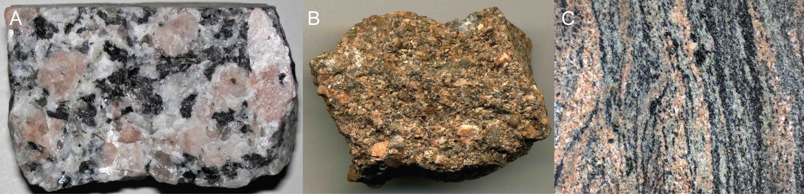
Minerals are the basic building blocks of rocks, which means rocks are made up of different combinations of minerals or just one mineral in some cases. Figure 2.1a is an example of a rock called granite, which is made up of a combination minerals. A mineral is a naturally occurring, usually inorganic, solid that can be defined by a chemical formula and a crystal structure. Figures 2.1b and 2.1c are two other types of rocks, sandstone and gneiss, that contain the same minerals as the granite in Figure 2.1a. Even though they contain the same minerals, all three of these rocks formed in different ways. We’ll get to that a little later, so for now, let’s focus on minerals.
2.2 Minerals
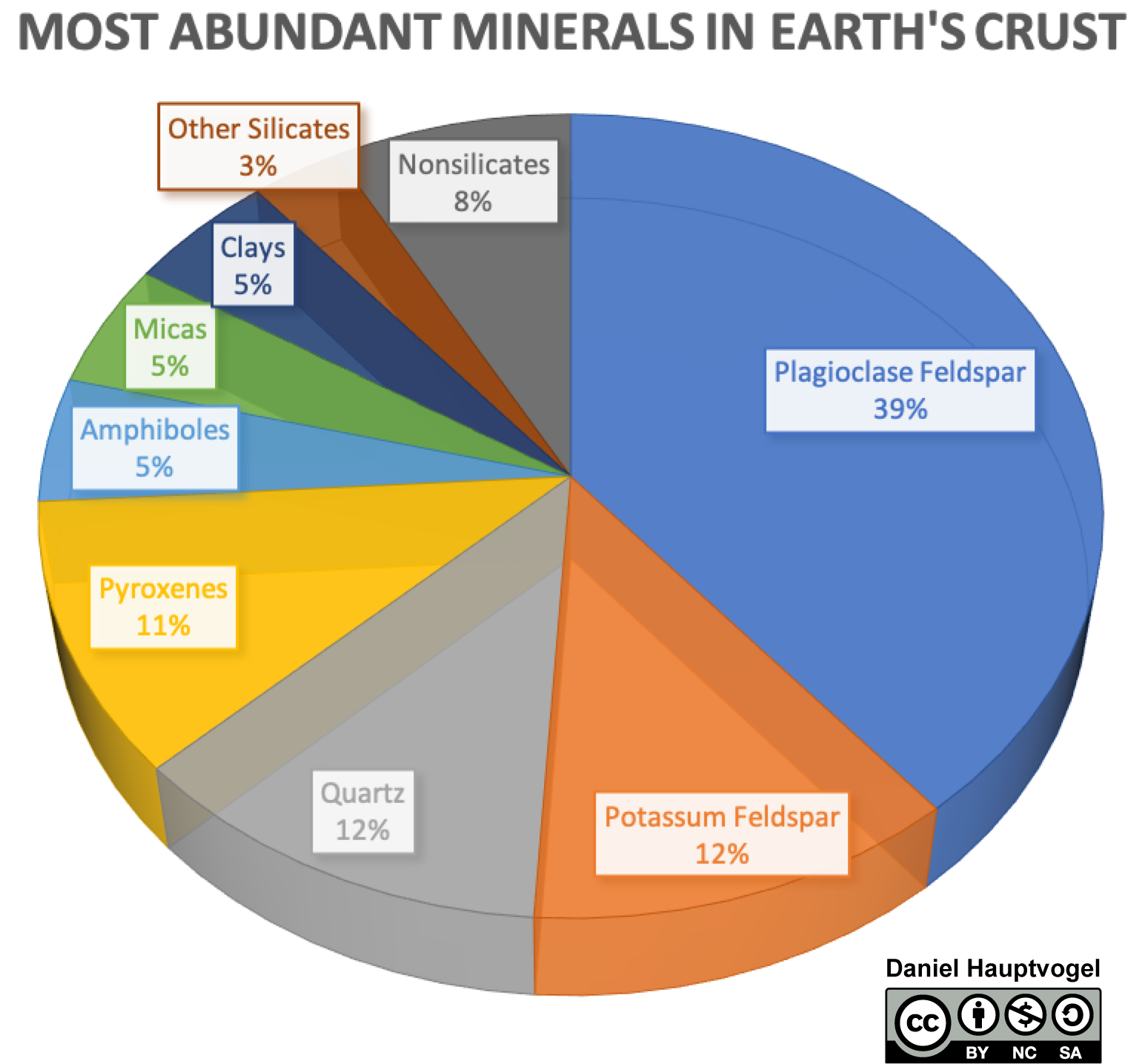
According to the International Mineralogical Association, there are 5,575 known minerals, but most rocks are composed of just a few common minerals. In fact, only seven minerals make up 84% of Earth’s crust (Figure 2.2). So when you find an unknown rock, there is a good chance that at least one of those seven minerals will be present.
Geologists can take rocks and minerals back to their laboratories and run in-depth chemical analyses to determine what minerals they have collected. You don’t have that luxury when you’re working in the field or the classroom, though. Instead, many minerals can be identified based on a few observable properties that don’t require high-tech, expensive equipment. So, distinguishing these seven common minerals and others is easier than you think. The common, observable properties of minerals are:
- Color
- Luster
- Streak
- Hardness
- Cleavage/Fracture
Color
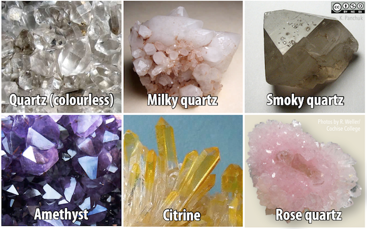
The color of minerals comes from small impurities in the chemical composition. Sometimes elements substitute for one another in the atomic structure of minerals, leading to significant changes in color. It is perhaps the most straightforward observable property, but it is rarely a diagnostic property for most minerals because the same mineral can come in various colors. Quartz, for example, can come in just about any color (Figure 2.3).
Luster
The term luster describes how light interacts with the surface of a mineral. There are many different terms used to describe the luster of a mineral, but for this lab manual, we are only concerned with metallic and non-metallic lusters (does it look like a metal or does it not look like a metal, respectively; Figures 2.4a and 2.4b). Be careful, though, because shiny doesn’t always mean it’s metallic. The technical difference between metallic and non-metallic is that metallic minerals do not allow light to pass through the atomic structure, and non-metallic minerals do allow some light to pass through.

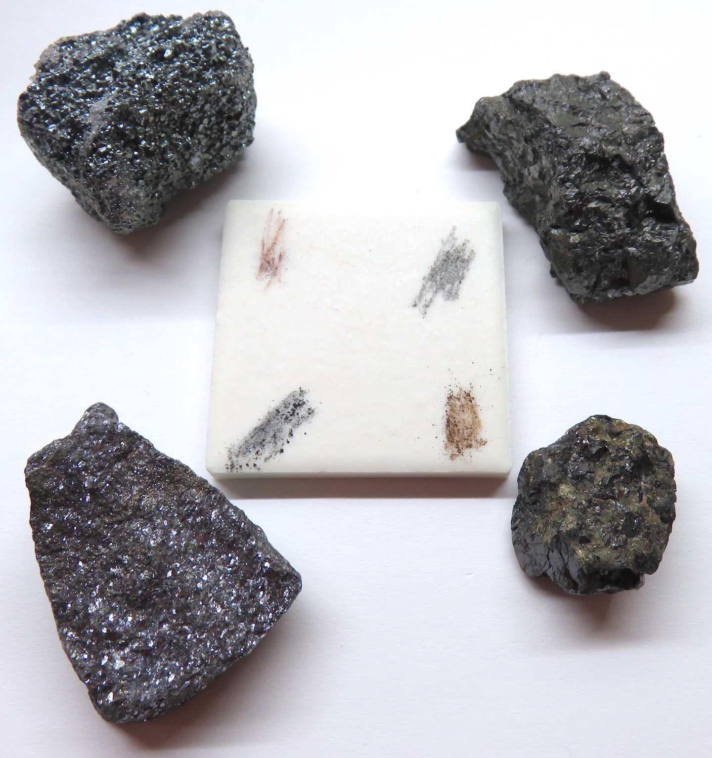
Streak
Streak is the color of a mineral in powdered form, which is observed by scratching the mineral across a ceramic streak plate (Figure 2.5). The powder color can be different from the mineral color because, when in powdered form, the mineral’s impurities do not significantly affect the absorption of light. The way light is absorbed and reflected is what gives things color. Streak is only a diagnostic property for metallic minerals because most other minerals have the same streak color as the hand-sample color or the streak is white.
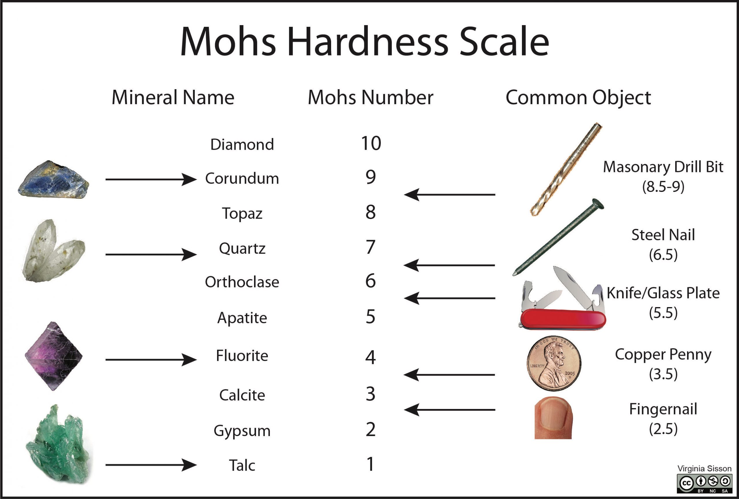
Hardness
The hardness of a mineral is a mineral’s ability to resist abrasion or scratching. Hardness is determined using the Mohs’ scale of mineral hardness (Figure 2.6), developed by Frederich Mohs in 1822. Mohs’ scale is qualitative, which means there is no quantitative relationship between hardness values; a 10 on the Mohs scale is not 10 times harder than a 1. The scale is based on the relative relationship between 10 different minerals.
How do you determine mineral hardness? When identifying mineral hardness in the classroom, you can use common objects with a hardness value defined on the Mohs scale. These common objects and their hardness are located on the right side of Figure 2.6.
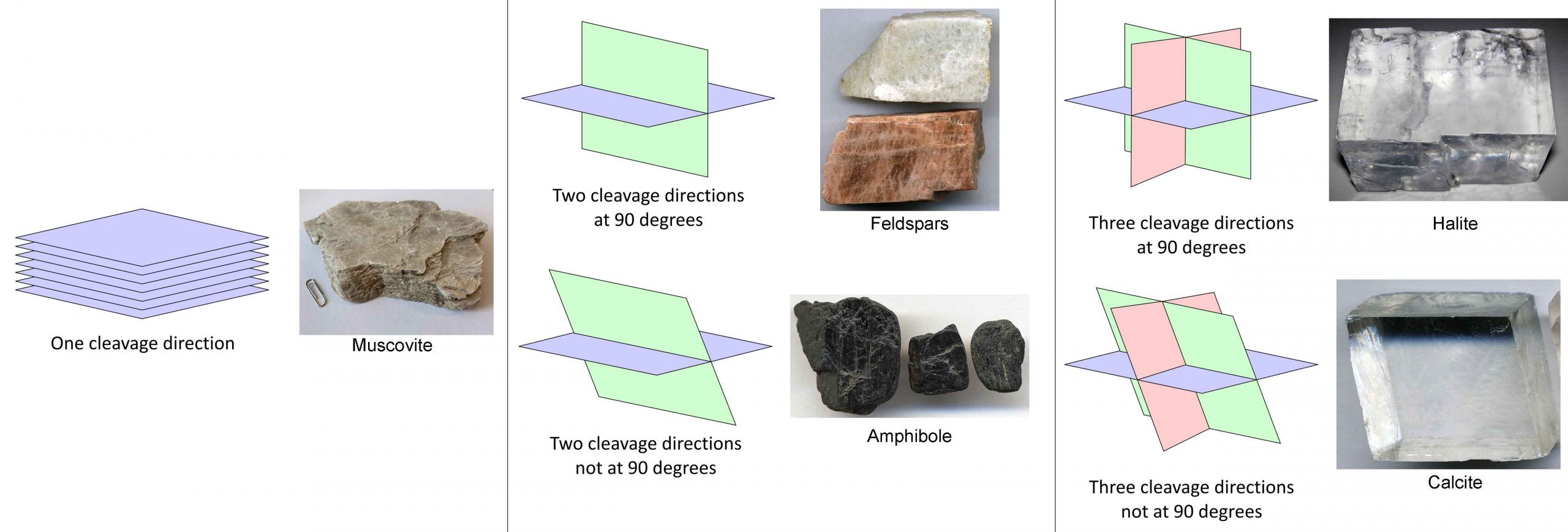
Cleavage/Fracture
Cleavage is a term used to describe minerals that break in a predictable way. When minerals break along planes in which chemical bonds are weak, they produce flat surfaces called cleavage planes. Minerals can have 1, 2, 3, or more planes of cleavage (Figure 2.7). When there is more than one plane, the angle between the planes can also be described. Cleavage is one of the most challenging concepts for introductory geology students, but it is a useful property to identify minerals. For example, amphibole and pyroxene have the same physical properties except for cleavage. Knowing whether a rock contains amphibole or pyroxene could reveal a lot about that rock’s geologic history, such as where and how it most likely formed.
While the concept of mineral cleavage is difficult, identifying cleavage in minerals doesn’t have to be. When looking at a mineral, the easiest way to identify cleavage is to shine a light on its surface. If that surface brilliantly reflects light, then you most likely have a cleavage plane. Today, just about everyone has a cell phone with a flashlight that can be used to identify cleavage. In the absence of that, you can move the mineral around underneath an overhead light or use sunlight.
Minerals don’t always break in predictable ways, and that’s when we use the term fracture. Fracture describes irregular breakage in minerals, which usually occurs on mineral planes that don’t have any weak bonds. This sounds easy enough; flat surfaces mean cleavage, and uneven surfaces mean fracture, but the truth is that it can be messy. Minerals can appear to have flat surfaces that are not actually cleavage, and fracturing can occur along planes of cleavage. This is why you need to look closely at the surface of a mineral using a hand lens.
A hand lens is a magnifying glass to help geologists look closely at rocks and minerals. To use the hand lens properly, you need to place the lens up against your face and then move the mineral or rock sample back and forth to get it into focus. A common mistake students make is holding the mineral or rock still and moving the hand lens; this is incorrect and will not help you see small-scale features in rocks and minerals.
Another thing that makes identifying cleavage difficult is the entire mineral sample does not have to take on the shape of the cleavages. The minerals in Figure 2.7 are examples where the samples do take on the cleavage shape, but this is not the case for most minerals. Instead, you need to use a hand lens to look at the small details of a single side of the mineral. There will be slight changes in the heights of the surface that you wouldn’t be able to see without the hand lens. It is along those “elevation” changes that you should be looking for signs of cleavage. Then repeat your examination on the other sides.
Exercise 2.1 – Identifying Common Minerals
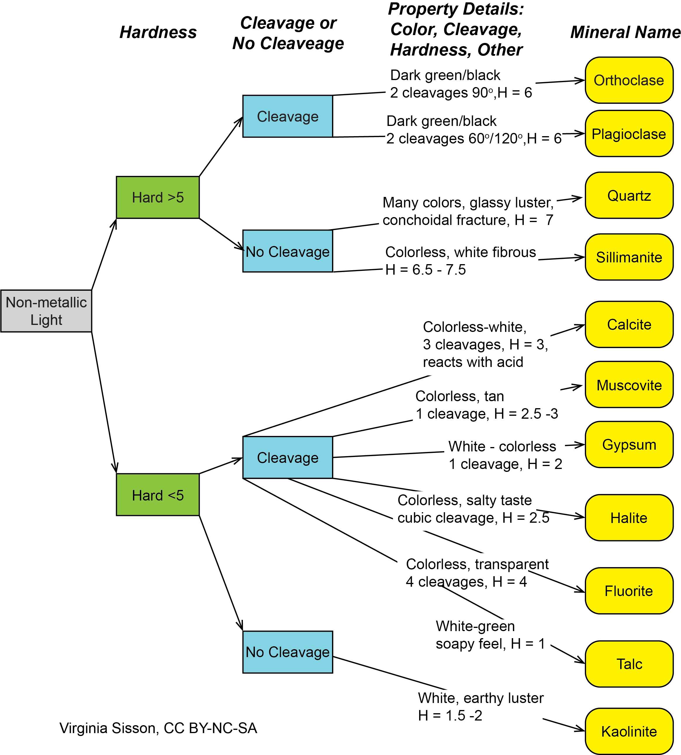
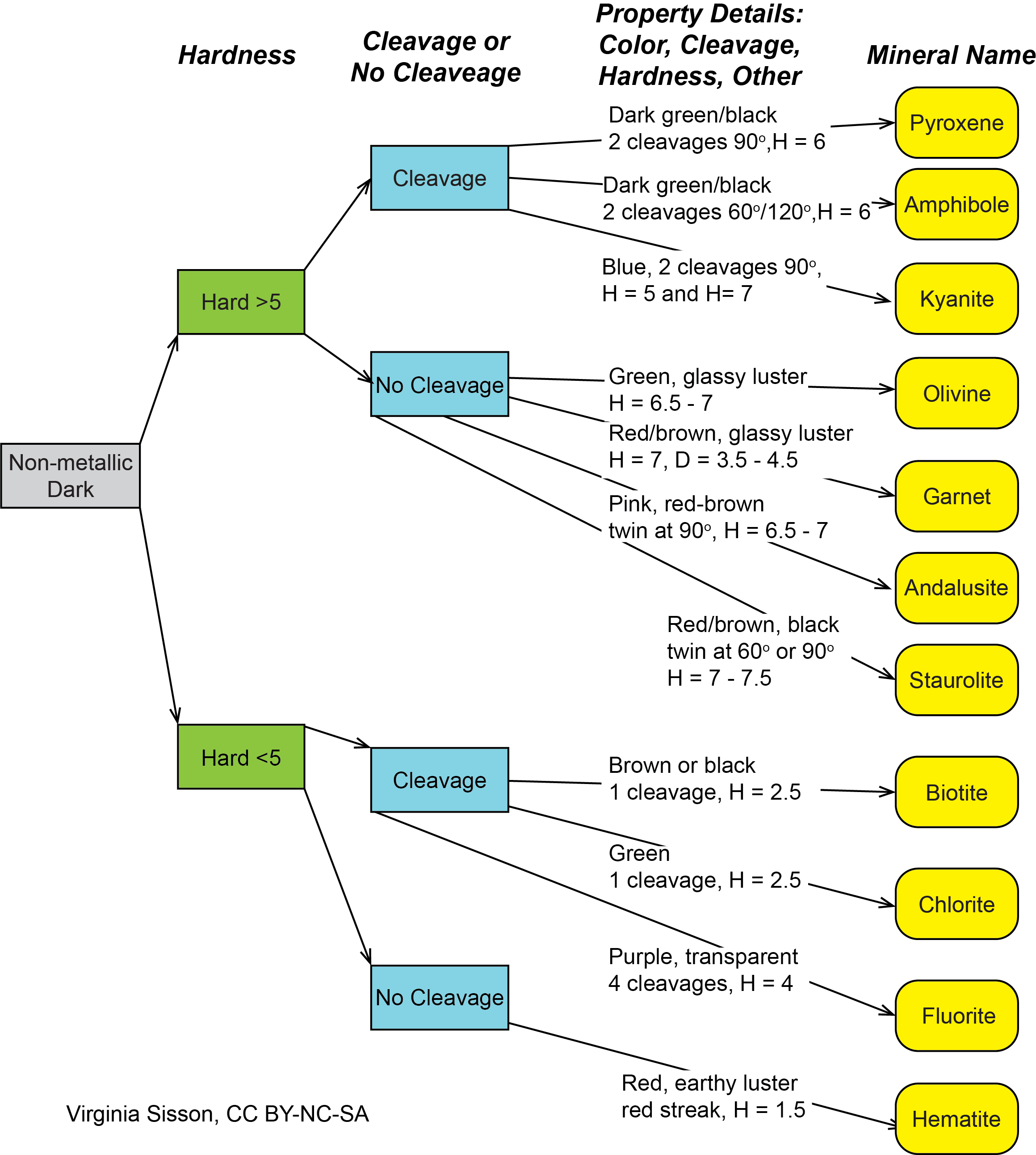
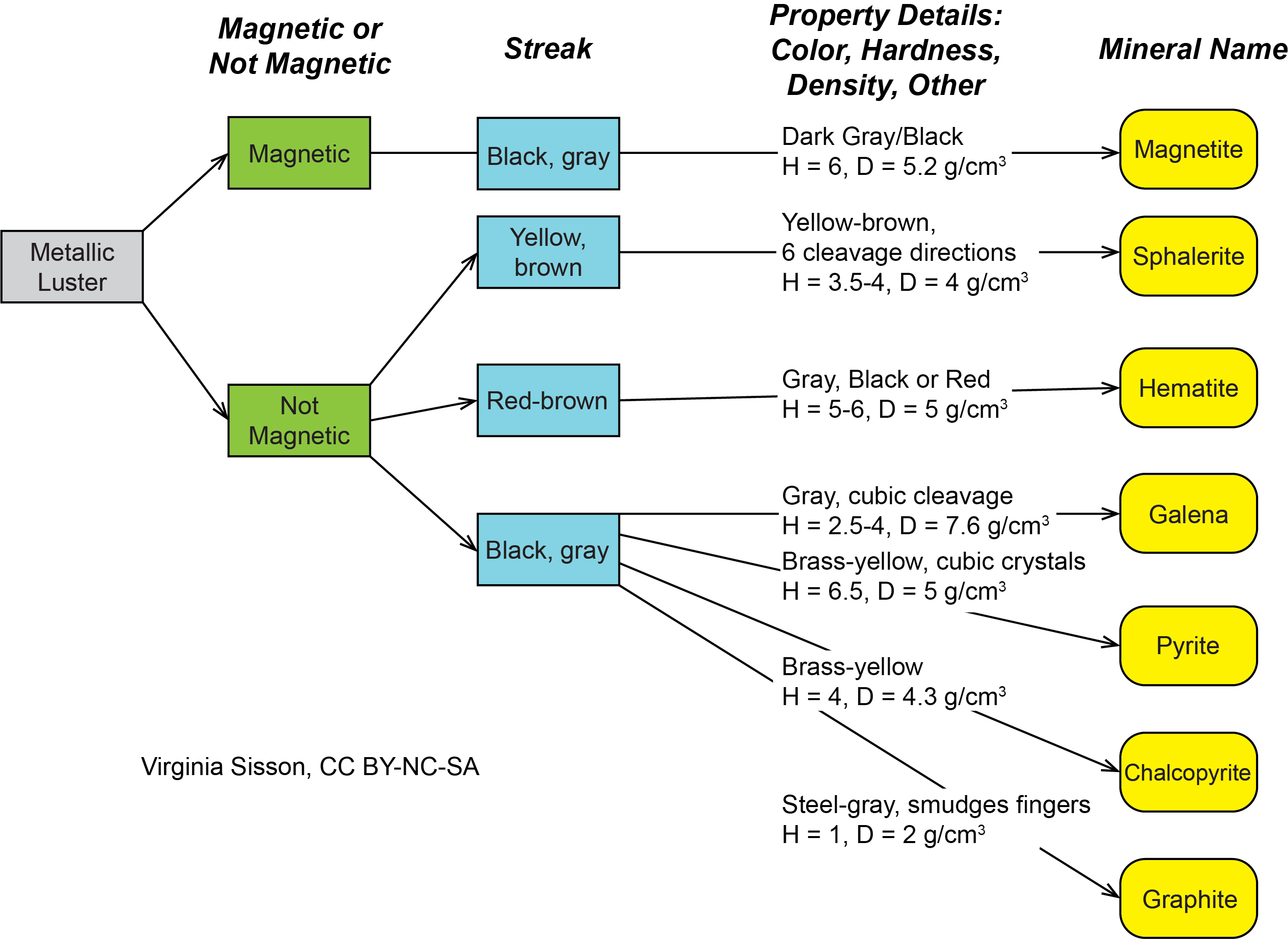
Your instructor will provide you with a set of unknown minerals. Identify each mineral based on its physical properties using either Table 2.1 as your guide or the mineral flow charts in Figures 2.8, 2.9, and 2.10. Fill in this information in Table 2.2. There are also many online guides to help you identify minerals, such as MineralID, Smart Geology (Android), or the app Mineral Identifier (Apple).
| Hardness | Color | Cleavage | Other | Mineral Name |
|---|---|---|---|---|
| 1-2 | Colorless | One plane | “Chewy” | Clays |
| 2-2.5 | Colorless, light tan, yellow | One plane | Can be peeled into transparent, flexible sheets | Muscovite |
| 2-2.5 | Brown, black, green | One plane | Can be peeled into thin, flexible sheets | Biotite |
| 2.5 | Colorless, white | Three directions at 90° | Cubic crystals, salty taste | Halite |
| 3 | Colorless, white | Three directions not at 90° | Rhombic crystals, reacts with HCl, double refraction | Calcite |
| 5-6 | Dark green to black | Two directions at ~60° and ~120° | Elongated crystals | Hornblende (Amphibole) |
| 5-6 | Dark green to black | Two directions at ~90° | Elongated crystals | Augite (Pyroxene) |
| 6 | Colorless, pink, gray | Two directions at 90° | Stubby, prismatic crystals | Potassium Feldspar |
| 6 | Colorless, white, gray, black | Two directions at 90° | Can have small grooves on one of the cleavages called striations | Plagioclase Feldspar |
| 6.5-7 | Green | No cleavage, can have conchoidal fracture | Stubby crystals or granular masses | Olivine |
| 7 | Mainly red and black | Conchoidal fracture | May occur in 12-sided, circular crystals | Garnet |
| 7 | Varied | Conchoidal fracture | May occur in six-sided, elongated crystals | Quartz |
| Sample ID | Color | Hardness | Cleavage | Mineral Name |
2.3 Rocks
Rocks are what most people think of when they hear “geology.” Rocks are made up of different minerals, and in some cases, just one mineral. Minerals in rocks can be difficult to identify, though. Even upper-level geology majors and practicing geoscientists can have trouble identifying minerals in rocks. Nonetheless, it is an essential skill to practice because it serves as one of the primary ways to identify rocks. When geologists go into the field to study rocks, one of the first things they do is get up close and personal with the rock, usually with a hand lens, and identify what minerals are present. Let’s practice with a simple exercise on identifying some common minerals in rocks in Exercise 2.2.
Exercise 2.2 – Identifying Minerals in Rocks
Your instructor will provide you with a selection of different rock samples. From the list of minerals in Table 2.3 below, indicate which rock sample(s) contain those minerals by filling out the “Rock Sample” column.
| Mineral | Rock Sample |
|---|---|
| K-feldspar | |
| Plagioclase feldspar | |
| Quartz | |
| Biotite | |
| Hornblende |
Based on how rocks are formed, geologists classify them into three basic types: igneous, sedimentary, and metamorphic. Igneous rocks form when magma or lava cools and solidifies. Minerals start to crystallize as the magma cools, and they interlock with each other in random orientations. Sedimentary rocks form when broken pieces of other rocks from weathering processes get cemented together. They can also form when minerals precipitate out of a solution, typically water, and are cemented together through sedimentary processes. Metamorphic rocks are pre-existing rocks that are altered by heat and pressure. Metamorphism often results in some type of pattern or orientation to the minerals, called foliation.
Exercise 2.3- Identifying Types of Rocks
Your instructor will provide you with a selection of unknown rocks. Using what you know about how each rock type forms, determine the rock type for each of your unknown samples and fill in Table 2.4.
| Rock Type | Sample |
|---|---|
| Igneous | |
| Sedimentary | |
| Metamorphic |
2.4 Igneous Rocks
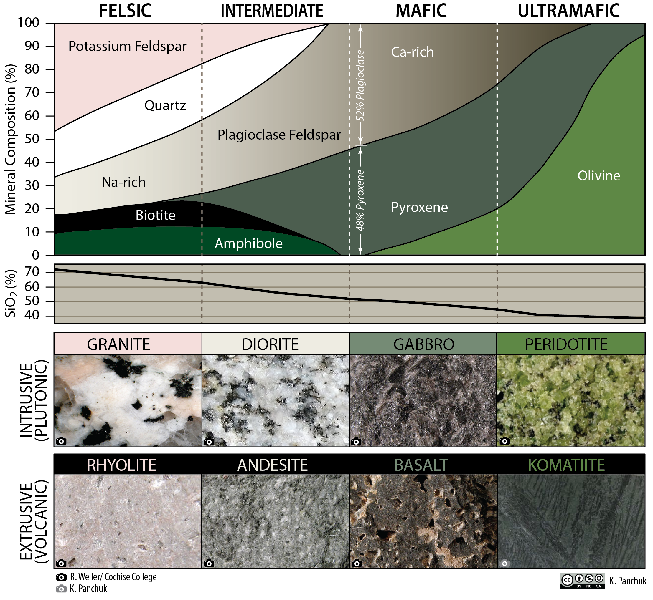
The classification of igneous rocks is based on chemistry and texture, which means it’s based on what minerals they have and how large the mineral grains are (Figures 2.11 and 2.12). The magma’s chemistry and temperature determine which minerals will form, and the size of the mineral grains is determined by how quickly the magma cools. Slow cooling rates (thousands to millions of years) make larger mineral grains. Fast cooling rates (days to hundreds of years) produce smaller grains. Igneous rocks with large grains are called intrusive or plutonic rocks, which means the magma cooled slowly within the Earth. Igneous rocks with tiny grains are called extrusive or volcanic because the lava cooled on the surface of the Earth. The distinction between small and large grains is whether you (or a well-trained geologist) can identify the minerals without using any magnification. Using this information, if you had a coarse-grained igneous rock that contained 10% quartz, 10% potassium feldspar, 50% plagioclase feldspar, 20% pyroxene, and 10% amphibole, it would be called a diorite. If the mineral grains were fine (small), the rock would be called andesite.
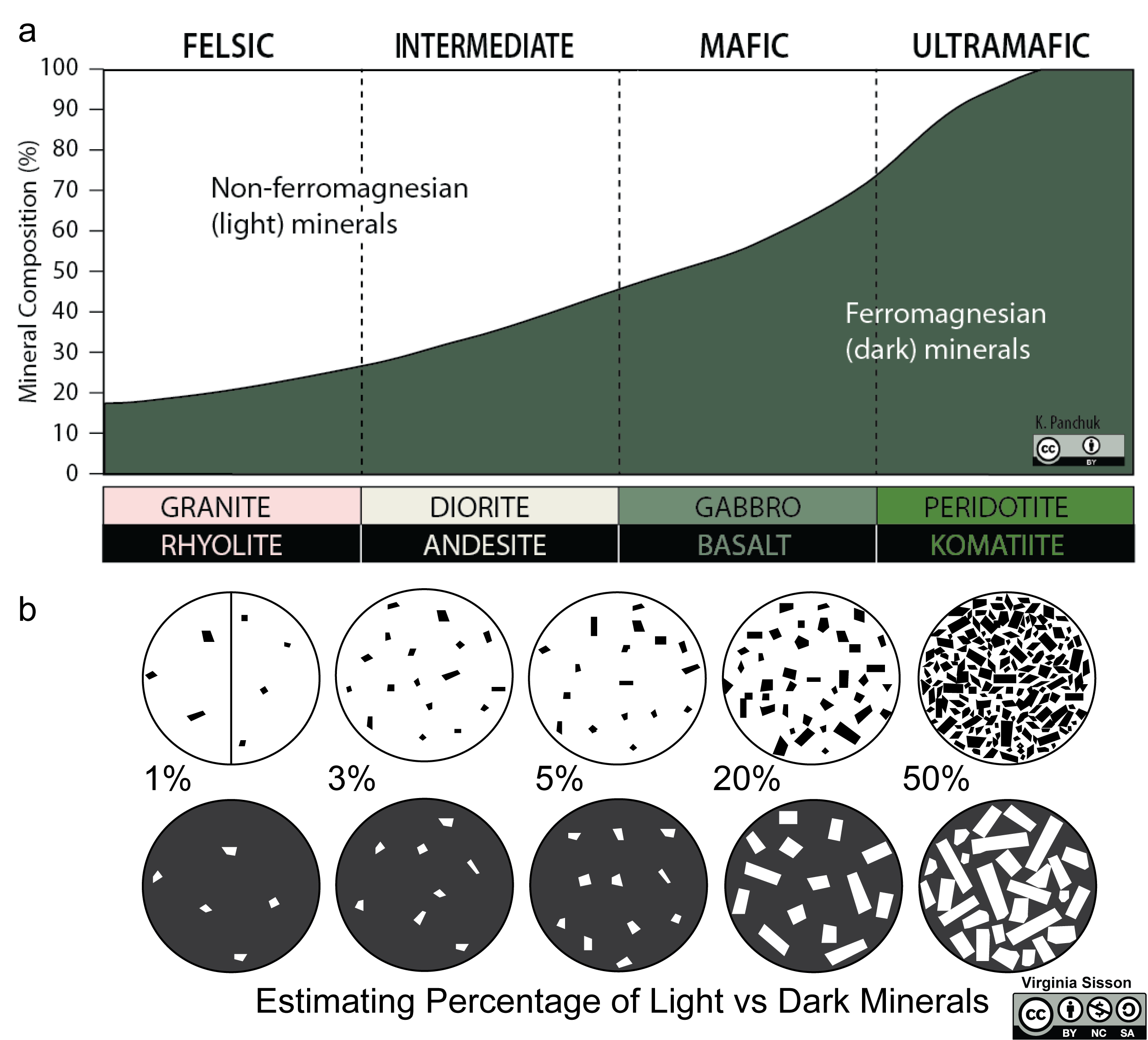
How would you identify minerals in an extrusive igneous rock if the grains are too small to see? There are a couple of tricks that geologists use to identify which type of igneous rock they have. Do you remember how color was not a diagnostic property for minerals? Well, color in an igneous rock can be diagnostic! Iron and magnesium-bearing minerals are darker in color, like olivine and pyroxene, and they are the primary minerals that makeup mafic and ultramafic igneous rocks. Potassium, aluminum, and silica-rich minerals, like quartz and potassium feldspar, are lighter in color and make up intermediate and felsic igneous rocks. Geologists can use the color of igneous rocks and the relative amount of light- vs. dark-colored minerals to help identify them (Figure 2.12).
Exercise 2.4 – Identifying Igneous Rocks
Your instructor will provide you with a set of unknown igneous rocks to identify. Use Figures 2.11 and 2.12 to fill out the information in Table 2.5.
| Sample | Intrusive or Extrusive | % Light vs. Dark Minerals (for intrusive) or Rock Color (for extrusive) |
Rock Name |
|---|---|---|---|
2.5 Sedimentary Rocks
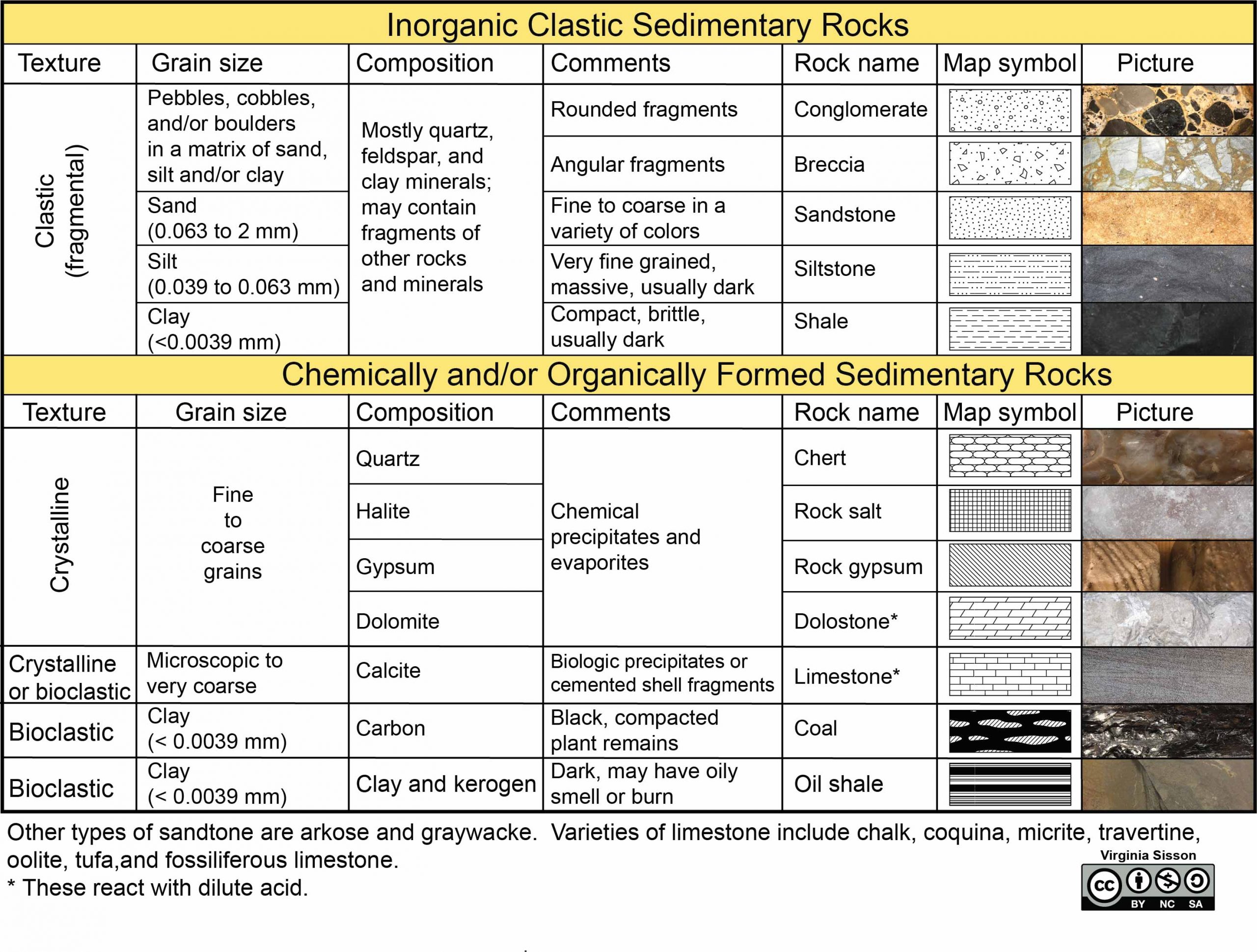
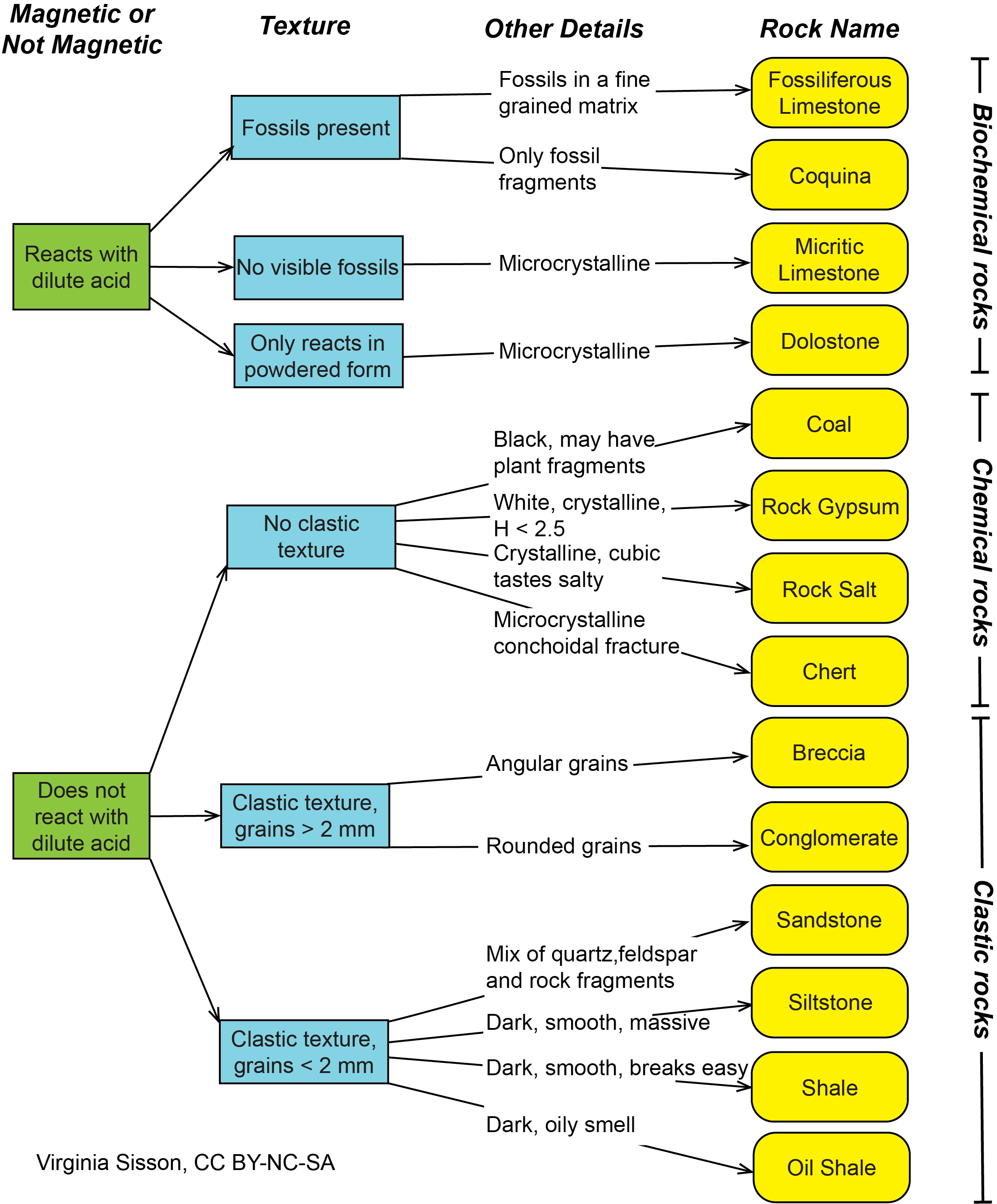
Sedimentary rocks can form in several ways (Figure 2.13) and are classified as clastic, chemical, and organic based on how they form. The most common way sedimentary rocks form is when other rocks weather into small particles and are transported by wind, water, or ice to an area where they are deposited and form layers. These are called clastic sedimentary rocks and are primarily classified based on their grain size. Sedimentary rocks can also form through chemical or organic processes. If you have a body of water containing dissolved salt and then that water evaporates, it will leave behind the salt as a solid mineral form called a precipitate, which is a chemical sedimentary rock. Organic sedimentary rocks form from the accumulation of organic debris. This organic material would need to be buried very quickly, so it doesn’t decay. Organic material in sedimentary rocks is where coal, oil, and natural gas come from. Then, there are sedimentary rocks that we can classify as biochemical. For example, foraminifera are tiny, single-celled organisms that build shells out of calcium carbonate. When they die, their shells can sink to the bottom of the ocean and accumulate to form a sedimentary rock. In this case, biological processes caused the chemical precipitation of the mineral for the shell, but it doesn’t contain organic compounds, so we call it bio-chemical.
In all cases, sediments need to be buried so the lithification process can take place. There are two steps involved in turning sediment into sedimentary rock; compaction and cementation. When grains are deposited, they typically have empty spaces between them called pores (porosity). Compaction reduces porosity by bringing the grains closer together. The best analogy to think about is your garbage can at home. When the garbage can is full, do you change the bag right away, or do you push down on it to create more room? By pushing down on trash, you reduce the space between the pieces of garbage and create more room at the top; this is compaction. Sediments work the same way, but what’s causing the compaction is the accumulation of more sediment on top of the previously deposited material. The more sediment that gets piled on top, the more compact the sediment beneath it becomes. Cementation is a process that happens during compaction. As sediments become compacted, water is squeezed out of the pore spaces. As the water leaves the sediment, it precipitates minerals into those pore spaces acting as a glue that holds the sediment together. The common minerals that make up the cement are calcite, quartz, and pyrite.
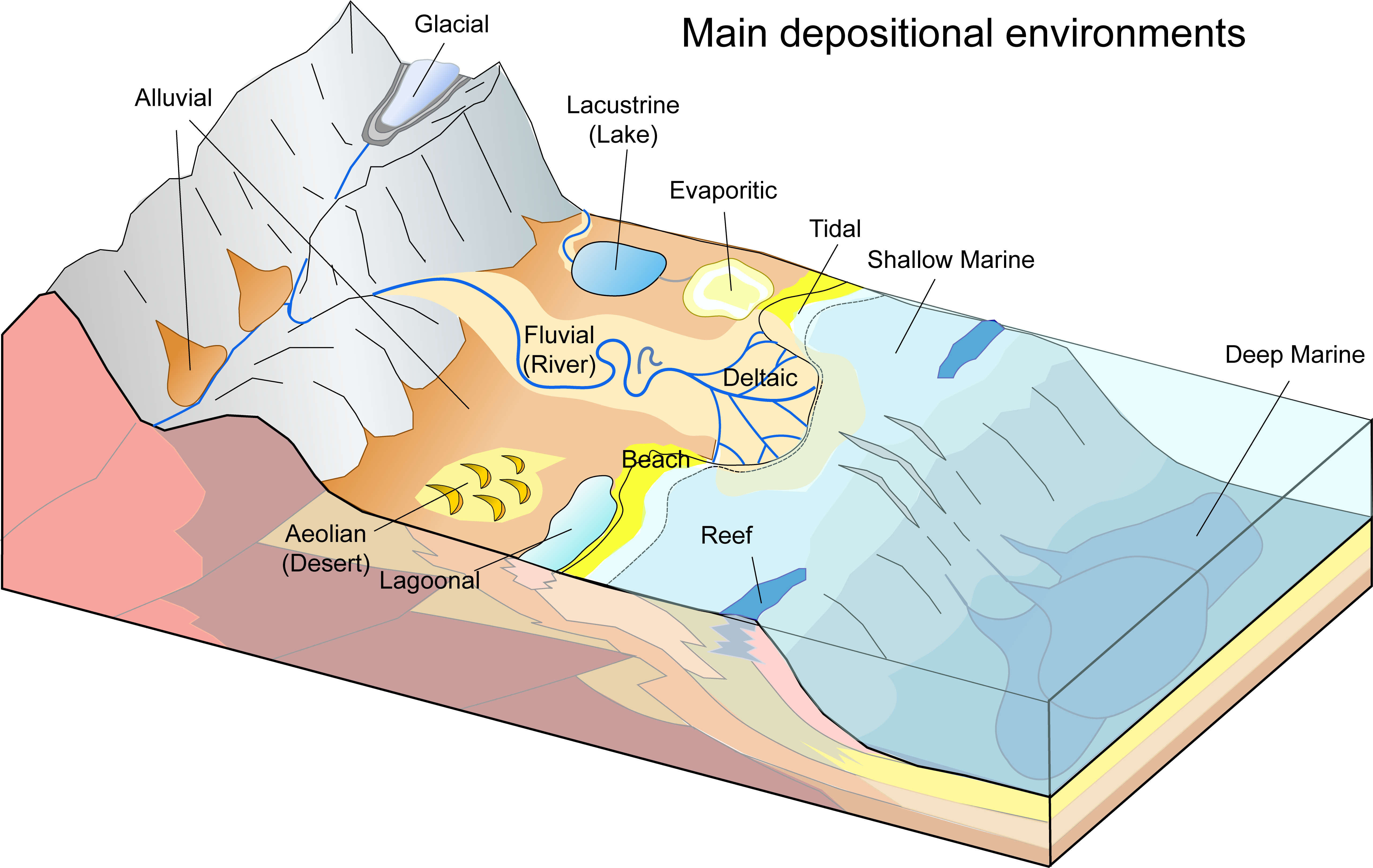
The locations where sediments are deposited are called depositional environments. There are a variety of depositional environments (Figure 2.14) that can be grouped into three broad categories: continental, marine, and transitional. Continental environments are areas where sediments are deposited on continents, marine environments are areas where sediments are deposited in the ocean, and transitional environments are coastal and tidal locations between continental and marine environments. Table 2.6 contains the most common environments, a brief description of them, and the common sedimentary rocks that can form in those environments.
| Environment | Description | Common Types of Sedimentary Rocks |
|---|---|---|
| Continental | ||
| Aeolian | Sediment deposited by wind; primarily deserts and coastal regions; well-sorted sand; typically red in color; variable energy. Example in Google Earth: Algeria. | Sandstone |
| Alluvial | Fan-shaped deposits caused by moving water; usually found in arid or semi-arid regions; contains gravel, sand, silt, and/or clay; poorly sorted; high energy; creates alluvial fans. Example in Google Earth: Death Valley National Park, California. | Conglomerate, breccia, sandstone, shale |
| Fluvial | Sediment deposited by moving water, primarily rivers; can contain gravel, sand, silt, and/or clay depending on how fast the water moves; variable energy; commonly red in color from oxidation. Example in Google Earth: Upper Mississippi River in Illinois/Missouri. | Conglomerate, sandstone, shale |
| Lacustrine | Lake settings that can contain sand, silt, or clay; generally low energy. Example in Google Earth: Lake Winnipesaukee, New Hampshire. | Sandstone, shale |
| Glacial | Sediment deposited by glaciers; variable grain sizes; poorly sorted. Example in Google Earth: Southern Patagonia, Argentina. | Conglomerate, breccia, sandstone, shale |
| Evaporitic | Forms where water evaporates and leaves behind mineral precipitates. Example in Google Earth: Utah. | Limestone, rock salt, rock gypsum. |
| Transitional | ||
| Beach | Along coastlines, sediment transported by wave action; contains well-sorted gravel and sand; high energy. Example in Google Earth: Island Beach State Park, New Jersey. | Sandstone |
| Deltaic | Where a river empties into a body of water; contains gravel, sand, and silt; low energy. Example in Google Earth: Yukon River, Alaska. | Sandstone, shale |
| Lagoonal | A shallow body of water separated from a larger body of water by barrier islands or reefs; very low energy; contains silt and clay. Example in Google Earth: East Matagorda Bay, Texas. | Limestone, shale, coal (swamps) |
| Tidal | Affected by the tides; mainly silt and clay; can create tidal flats; low energy. Example in Google Earth: Bay of Fundy, Nova Scotia. | Shale |
| Marine | ||
| Shallow | Located on the continental shelf; mainly sand and silt; energy decreases with distance from shore. Example in Google Earth: Eastern Gulf of Mexico. | Sandstone, shale, limestone |
| Deep | The deep ocean; very low energy; mainly clay; can contain turbidite deposits of variable sediment sizes. Example in Google Earth: Pacific Ocean. | Shale, chert, limestone |
| Reef | A bar of rock, sand, or coral. Example in Google Earth: Great Barrier Reef, Australia. | Limestone |
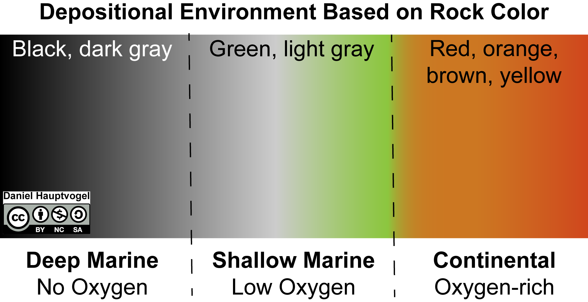
You’ll notice that the same type of sedimentary rock can be found in many different settings, making it difficult to determine the depositional environment. Sometimes, the color of a sedimentary rock can indicate the depositional environment because the color is largely determined by how much oxygen is available as the sediment is buried and lithified (Figure 2.15). Reddish colors can indicate oxygen-rich continental environments, like a flowing river or desert. Green and light gray colors mean low oxygen, which can be found in shallow marine environments. Black color means no oxygen, which would indicate a deep marine or swamp environment. Color is not always a good indicator, though, because the sediment only alters its color after burial. The conditions affecting buried sediment may not always match the environment on the surface above it.
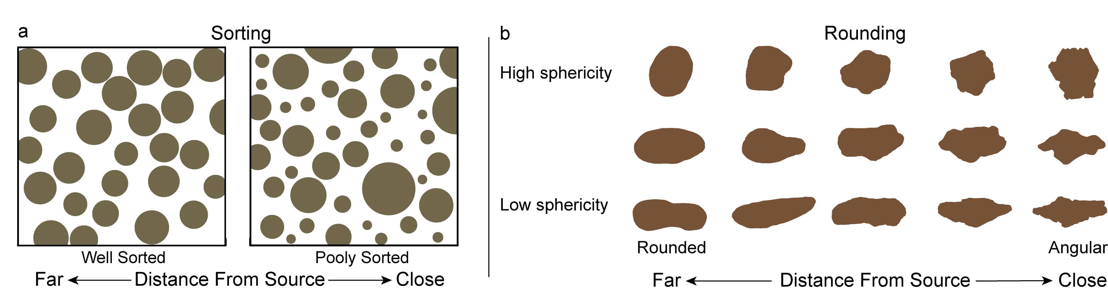
The size and shape of grains within sedimentary rocks can also help you interpret that sediment’s history (Figure 2.16). When all of the grains in the rock are about the same size, it is called well-sorted. Usually, sediment needs to travel a far distance from its source to be well-sorted. In contrast, poorly sorted sediment is very close to its source. The rounding of sediment grains is also an indicator of how far the sediment traveled. Grains that have smooth edges are considered well-rounded and have traveled a far distance. These grains start out with rough edges and become smoother as they travel further and further. In contrast, grains with sharp edges are considered angular and have not traveled a far distance.
Exercise 2.5 – Identifying Sedimentary Rocks
Your instructor will provide you with a set of unknown sedimentary rocks to identify. Use Figures 2.13 to 2.17 and Table 2.2 to fill out the information in Table 2.7 below.
| Sample | Clastic, (Bio-) Chemical, or Organic | Rock Name | Possible Depositional Environments |
|---|---|---|---|
2.6 Metamorphic Rocks
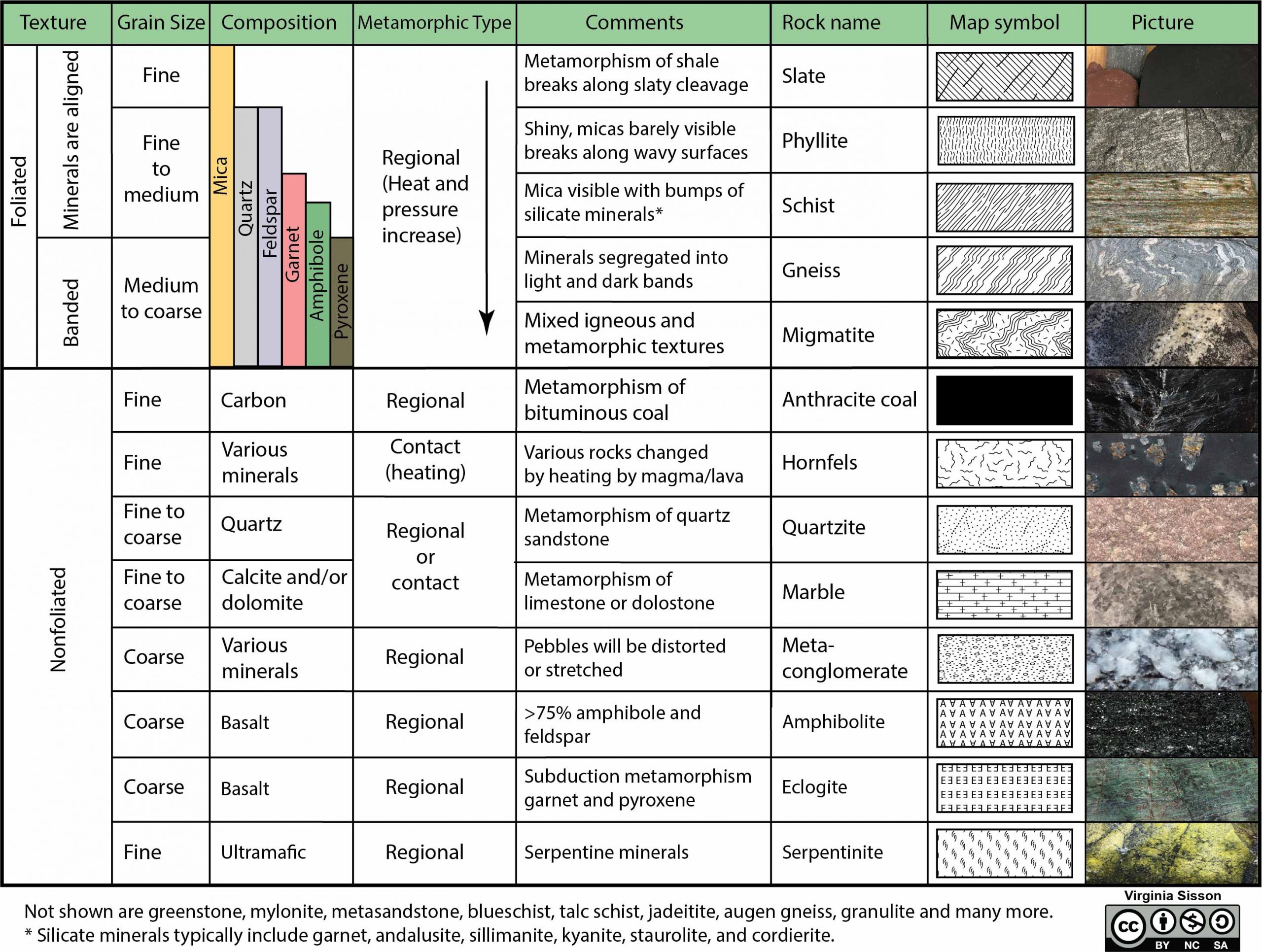
Metamorphic rocks (Figure 2.18) form when any pre-existing rock is altered by heat and/or pressure. The two sources of heat for metamorphism are the heat from a magma chamber and the geothermal gradient, which is the natural increase in temperature when getting deeper into the Earth. Pressure also increases with depth in the Earth, but intense pressure also occurs during tectonic plate collisions. This is why most of the world’s metamorphic rocks are found in mountain belts or ancient mountain belts.
Heat and pressure can cause several changes in rocks, such as recrystallizing minerals, creating new minerals, and orientating minerals in a direction perpendicular to pressure. The orientation of minerals is the most noticeable feature when recognizing metamorphic rocks. Heat works to “soften” minerals, allowing ions to begin migrating in and out of crystal structures. Then pressure forces the minerals to re-orientate. Heat is the most important factor, though; without heat, the rock would just break under intense pressure. When minerals take on some type of orientation due to metamorphism, it’s called foliation. As pressure increases, so does the degree of foliation. Not all metamorphic rocks exhibit foliation because some minerals change very little under metamorphic conditions (quartz, for example); these types of metamorphic rocks are called non-foliated or massive and can be very difficult to tell apart from igneous rocks.
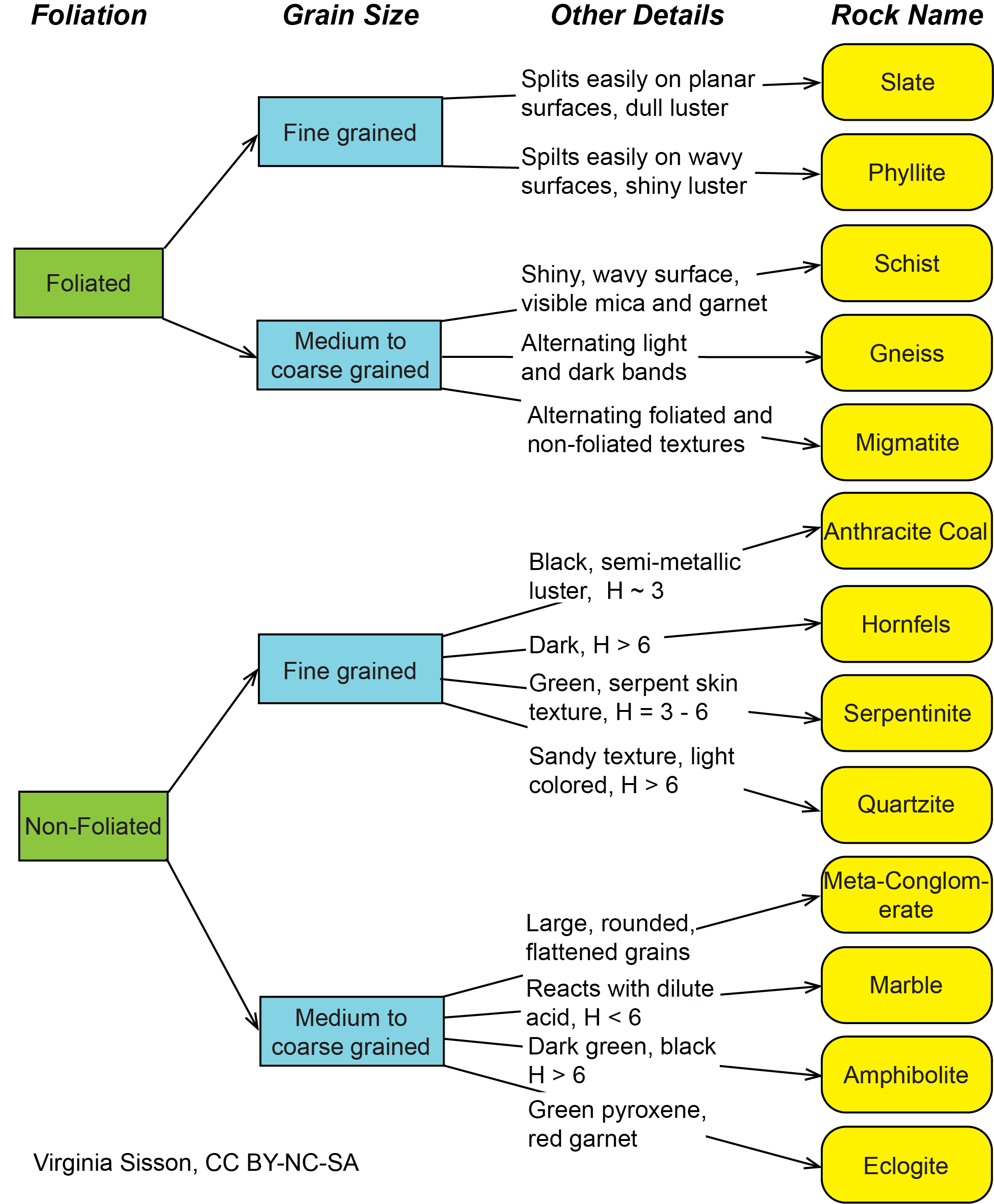
The pre-existing rock, before metamorphism occurred, is called the protolith. If you’ve taken an introductory Physical Geology class, you learned to differentiate metamorphic rocks mostly by their texture and classified them as slate, phyllite, schist, and gneiss. You may have even been introduced to the term migmatite for rocks that had both igneous and metamorphic textures as these were starting to undergo partial melting. These textural terms are associated with changes in metamorphic temperature and pressure, often referred to as the metamorphic grade or just grade.
Confused by metamorphism? Don’t feel alone, as many students and even professional geoscientists have difficulties describing and interpreting metamorphic rocks. First, you need to understand all factors affecting igneous and sedimentary rocks. Then, you add the effects of heat and/or pressure, but unlike other rocks, this can vary dramatically across a region. Often there has been more than one tectonic event in that region, adding even more complications for you to interpret. It is akin to understanding a four- or five- dimensional image and difficult to comprehend all the factors at once. You may want to review your Physical Geology lab and text before tackling metamorphic rocks and these exercises.
Exercise 2.6 – Identifying Metamorphic Rocks
Your instructor will provide you with a set of unknown metamorphic rocks to identify. Use Figures 2.18 and 2.19 to fill out the information in Table 2.8.
| Sample | Foliated or Non-foliated | Rock Name | Protolith |
|---|---|---|---|
Let’s build on your metamorphic rock foundation and start to interpret metamorphic rocks using mineral assemblages. To do this, you have to start by knowing the protolith (parent) material for the metamorphic rock. If you can distinguish mafic (basaltic protoliths) from shale (sedimentary protoliths), this will be easy.
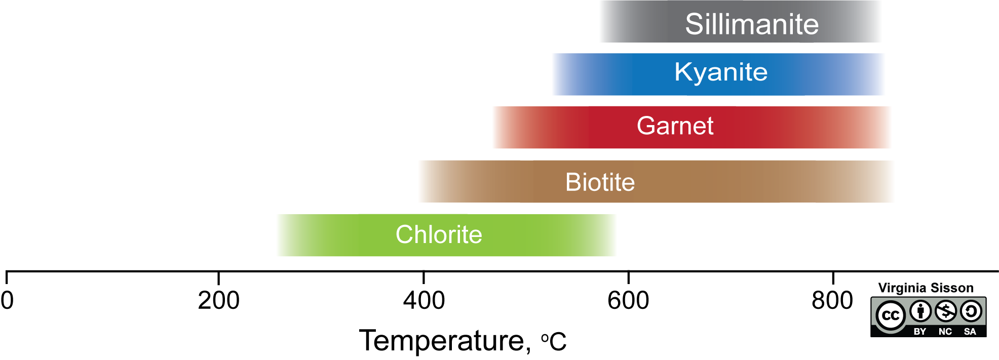
During metamorphism, rocks with a shale protolith will always have quartz, feldspar, and muscovite mica. So, you are on the lookout for new minerals, often seen as porphyroblasts. Most of these are not taught in Physical Geology, so here are some minerals you will need to know: chlorite (a dark green mica), biotite, cordierite, garnet, staurolite, sillimanite, kyanite, and andalusite (Figure 2.20). The last three minerals on this list you may remember are polymorphs: minerals with the same composition but unique internal structures (Figure 2.21). If you can identify these alumino-silicate minerals in a schist or gneiss, then you can determine the pressure-temperature conditions for that terrane. In general, rocks with kyanite and sillimanite are found in areas that have undergone continent-continent collision and are considered medium-pressure terranes. In contrast, areas with andalusite and sillimanite have an elevated geothermal gradient in response to either divergent zones or unusual ocean-continent collision zones called low-pressure terranes.
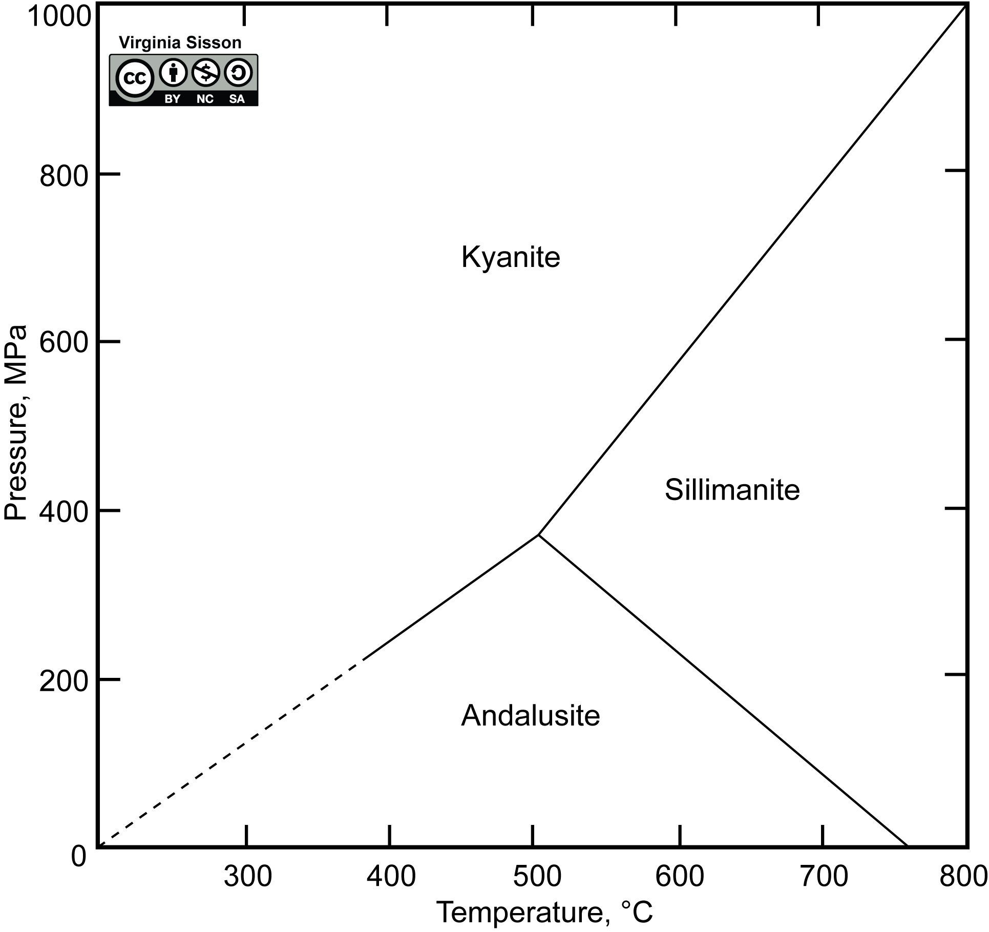
During a continental collision, the sequence of metamorphic rocks that form can be predictable by following the Barrovian sequence (Figure 2.22). Basically, the further away from the collision or the higher up in the crust the rock is, the lower the grade of metamorphism, while the closer and deeper the rocks are, the higher the grade. So, how do these deeper, high-grade metamorphic rocks become exposed at the surface? The answer is erosion; the low-grade rocks above need to be removed to expose the high-grade rocks below. This is relatively easy for an uplifting mountain belt because the increased surface area of the mountain allows more weathering and erosion to occur. If you are looking for exposures of high-grade metamorphic rocks, your best chance of finding them is near the center of the collision, where much of the uplift and erosion took place. The Barrovian sequence pattern is when the grade of metamorphic rocks increases as you approach the collision center, reaching the highest grade near the center and then decreasing in grade as you move to the other side (like a mirror image). Of course, this perfect, mirror-image pattern is not always seen because the rocks may not be exposed, or maybe faults have moved rocks from their original positions, or there was significant variability in pressure-temperature conditions.

Exercise 2.7 – Understanding the Barrovian Sequence
Continental collision and closure of the Iapetus Ocean in the Ordovician and early Devonian resulted in the Caledonide Orogeny. By the way, Caledonia is Latin for Scotland. One of the hallmarks of continental collision are suites of metamorphic rocks such as you’ve been looking at in Exercise 2.6.
Now let’s put together information from the rocks you’ve looked at with a map of the metamorphism of the Scottish Highlands. British geologist George Barrow mapped the area in Figure 2.23 in the 1890s. He realized that he could distinguish metamorphic zones by using their mineral assemblages. One more clue you need to solve this exercise is that there is a relationship between pressure and depth in the Earth as 300 MPa corresponds to approximately 10 km depth. So, you can convert the depths in Figure 2.22 to pressure with this approximation.
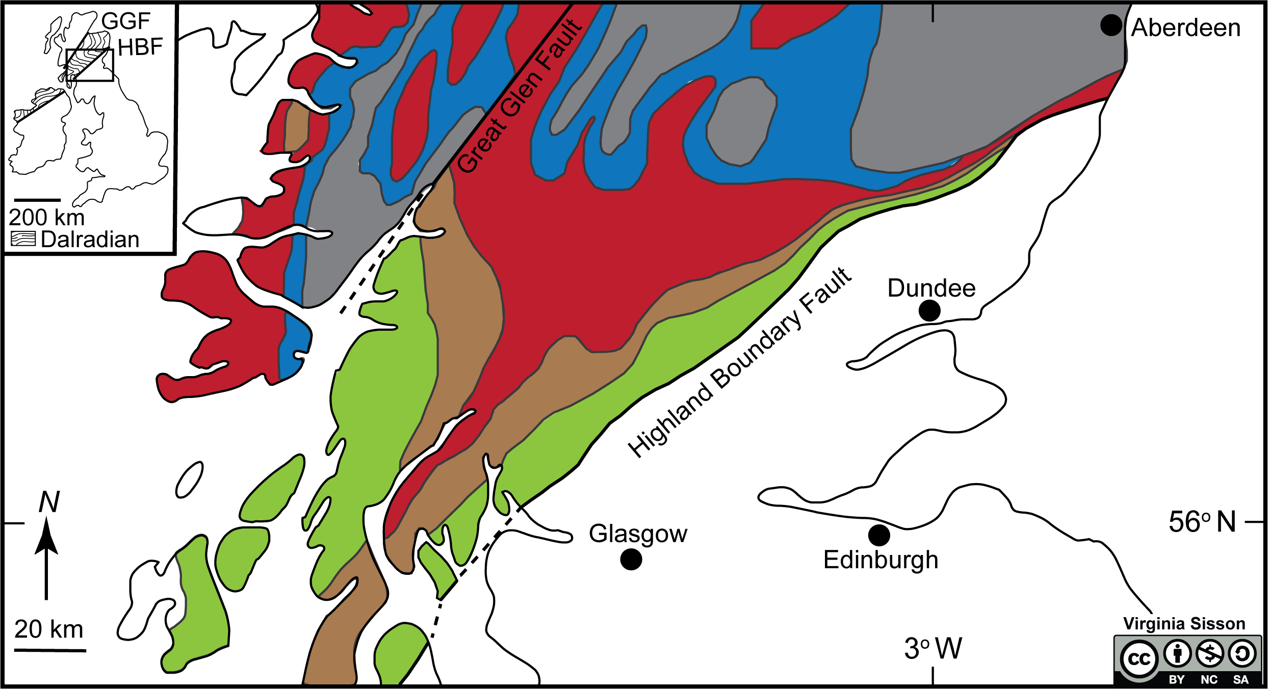
- Label the colored areas on the map with the mineral present according to the scheme used in Figure 2.20.
- Where on this map do you think your samples from Exercise 2.6 occur?
- On the map, mark which areas you think represent the shallowest and deepest during metamorphism.
- Draw a line on the map that corresponds to only a change in temperature.
- On the cross-section shown in Figure 2.22, plot an approximate path through the metamorphic zones. It will be up to you to decide how your metamorphic rocks evolved and your path may be different from a colleague’s.
- To help understand the metamorphic history of a region, geologists will construct geodynamic models of how heat and pressure in the Earth evolve through time. These models start with an initial set of conditions for the area. In Figure 2.22, the heavy black lines show two continental plates colliding; each has an initial lithosphere thickness of ~ 35 km. The convergence causes deflection of the Moho (Mohorovičić) discontinuity between the crust and mantle. Over time, the temperature readjusts. The colored areas on this plot show the metamorphic assemblages about ~35 million years after collision (Lyubetskaya and Ague, 2010). The first step to using this diagram is to convert metamorphic depths to pressures. A good rule of thumb is that 3 km depth is ~100 MPa. Use your results from part e to fill in Table 2.9.
Table 2.9 – Worksheet for Exercise 2.7f Metamorphic Zone Depth Pressure Temperature Chlorite Biotite Garnet Kyanite Sillimanite - Using your calculated pressures from Table 2.9, draw a line on Figure 2.21 that corresponds to your sequence of metamorphic assemblages from the map. This is called a pressure-temperature (PT) path. Geologists now like to add geochronology constraints (t), deformation (d) or compositional constraints (x), so you’ll hear them discuss PTt, PTtd or PTx paths when trying to determine the tectonic history of a region.
2.7 Using Rocks to Interpret Earth’s History
Igneous, sedimentary, and metamorphic rocks can all be used to interpret Earth’s history. Igneous rocks can help determine the plate tectonic setting of an area, sedimentary rocks help determine the environment of an area, and metamorphic rocks provide information about rocks before their deformation and the tectonic setting. All the following exercises will use your critical thinking skills.
Exercise 2.8 – Interpreting Volcanic History
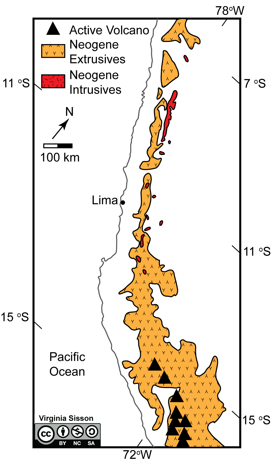
There are a few places on Earth with significant mountainous relief as well as igneous activity. One such place is the western margin of South America, which has been the site of ocean-continent convergence since the Jurassic (~185 Ma). Thus, it has a long history of almost continuous subduction-related volcanism and igneous activity. In the Central Andes Mountains, igneous rocks formed during the Neogene portion of geologic time between 23 and 2.5 million years ago; these include both intrusive and extrusive rocks (Figure 2.24). These volcanic rocks are overlain by more recent volcanoes.
- In the suite of igneous rocks provided by your instructor, which rocks are most closely associated with the Neogene intrusives?
- Which rocks would be associated with the Neogene extrusive volcanic rocks?
- Would the same rock types be found in the active volcanoes?
- Describe at least three differences between the map patterns of the recent volcanoes, Neogene extrusives, and Neogene intrusives.
- Critical Thinking: What can explain some of these differences in the map patterns?
Exercise 2.9 – Rocks of the Grand Canyon
The Grand Canyon has amazed tourists and geoscientists alike, not only for its beauty but by the fantastic stratigraphic sections (layers of sedimentary rock) exposed in its walls. The South Rim of the Grand Canyon is composed of metamorphic, igneous, and various sedimentary rocks. Go here if want to see representative samples of some of these rocks. Figure 2.25 shows a stratigraphic column of the Grand-Canyon (see Figure 0.3 for a sketch of the Grand Canyon).
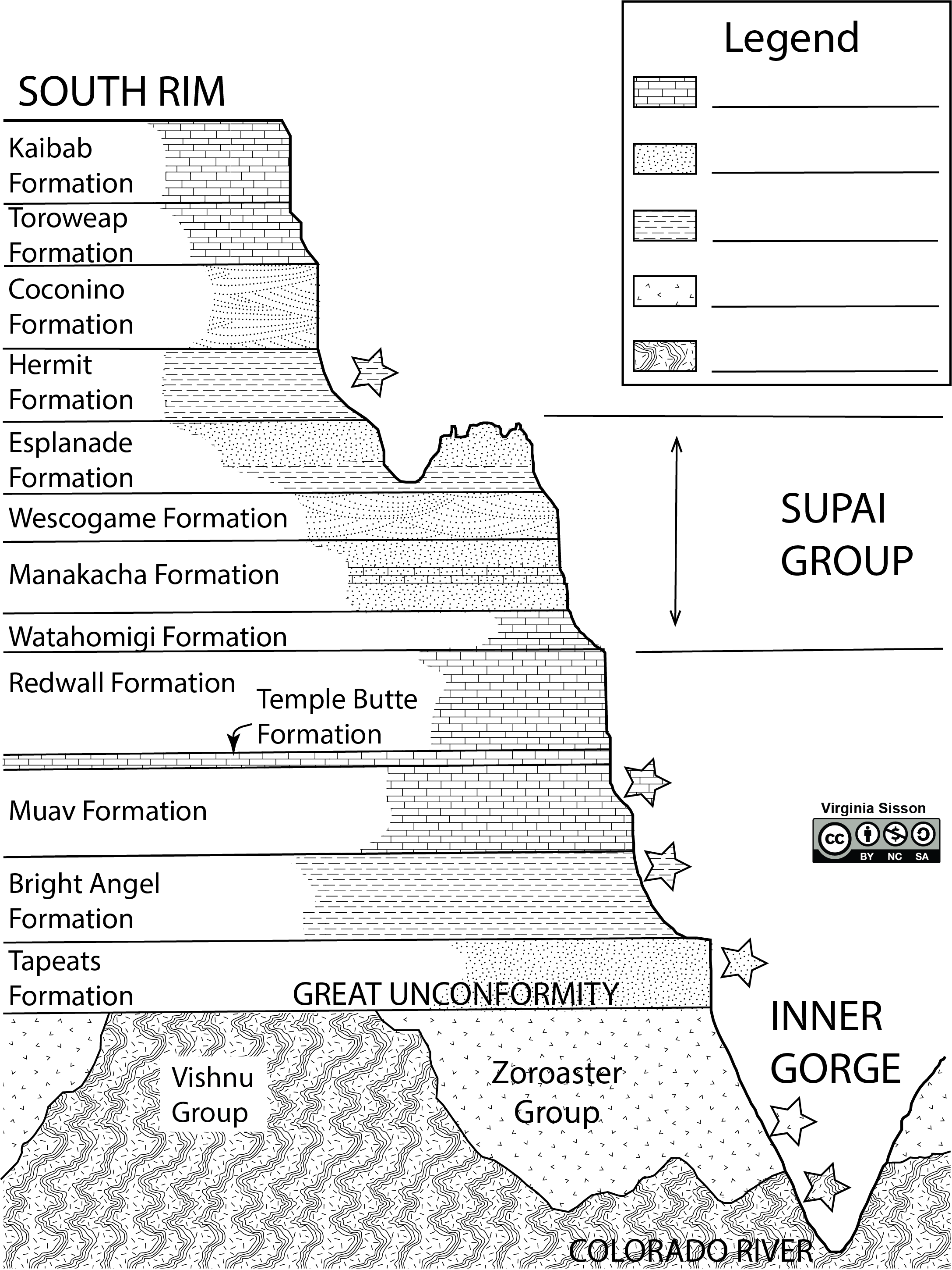
Table 2.10 contains descriptions of some of the different rocks found in the Grand Canyon.
- Which rocks from your kit resemble the sedimentary units marked with a star on the Grand Canyon stratigraphic section? Fill this out in the third column of Table 2.10.
- The symbols used to describe these rocks are standardized. Based on your findings from part a, complete the legend in Figure 2.25 by identifying the type of rock each symbol stands for.
| Rock Formation* | Description | Matching Rock From Your Kit |
|---|---|---|
| Vishnu Group | Group of foliated metamorphic rocks that are the result of various rocks, mostly igneous, being exposed to high degree metamorphism. | |
| Zoroaster Group | Igneous rocks composed of coarse-grained intrusions composed mostly of feldspar and quartz, with minor hornblende and biotite. | |
| Tapeats Formation | Composed mostly of sand-sized quartz grains with medium roundness. It is mostly massive, but bedding is visible in some areas. | |
| Bright Angel Formation | Composed of fine-grained shale, and trilobite fossils are common within this unit. | |
| Muav Formation | Chemical and biochemical sedimentary rocks that react with dilute acid. | |
| Hermit Formation | Extremely fine-grained, dark-colored sedimentary rocks which have easily observable bedding. Most minerals are clay minerals but can’t be observed, even with the help of a hand-lens, due to their extremely fine grain size. |
*See this Wikipedia entry for the differences in stratigraphic unit terminology.
Most of the rocks formed at divergent plate boundaries are igneous, with a thin layer of deep marine sediments on top. Since these sediments accumulate in the deep ocean far from the continents, there are only chert and marine clays. However, there are significant accumulations of igneous rocks derived from the decompression melting of Earth’s peridotite mantle. Do you recall what kind of rock forms from the partial melting of an ultramafic rock? It will be a mafic rock, either extrusive or intrusive. The oceanic crust is subdivided into five layers, as shown in Figure 2.26. This entire sequence is called an ophiolite. Ophiolites are typically exposed on Earth’s surface during the end of the subduction process as two continents move closer together and collide. During these final stages of subduction, the oceanic lithosphere gets stuck in the middle of the continental collision and is uplifted with the newly forming mountain belt. This is why most ophiolites are found in mountains.
Exercise 2.10 – Ophiolites
Ophiolites offer clues to where oceanic crust used to exist, and they help geologists understand processes at mid-ocean ridges.
- Your instructor has given you a suite of rocks that represent different layers in an ophiolite sequence. Identify your rocks and complete the legend at the bottom of Figure 2.26 by filling in the compositions and rock names.
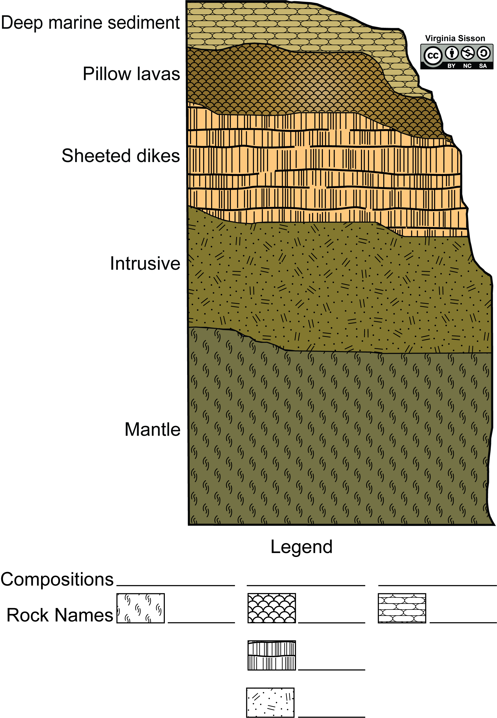
Figure 2.26 – Sequence of rocks in an ophiolite complex. Since it is difficult to find a location with all of these igneous rock types exposed in one outcrop, this is a composite of several different ophiolite exposures. The patterns used for the different units are adapted from the U.S. Geological Survey. Since most ophiolite sequences are composed primarily of mafic to ultramafic igneous rocks underneath deep marine sediment, we used dark green to brown colors for the different rock types. Image credit: Virginia Sisson, CC BY-NC-SA. - Explain why ophiolites show a sequence that moves from intrusive rock to extrusive. Hint: Think about relative cooling rates.
- What do pillow lavas tell you about where they were formed?
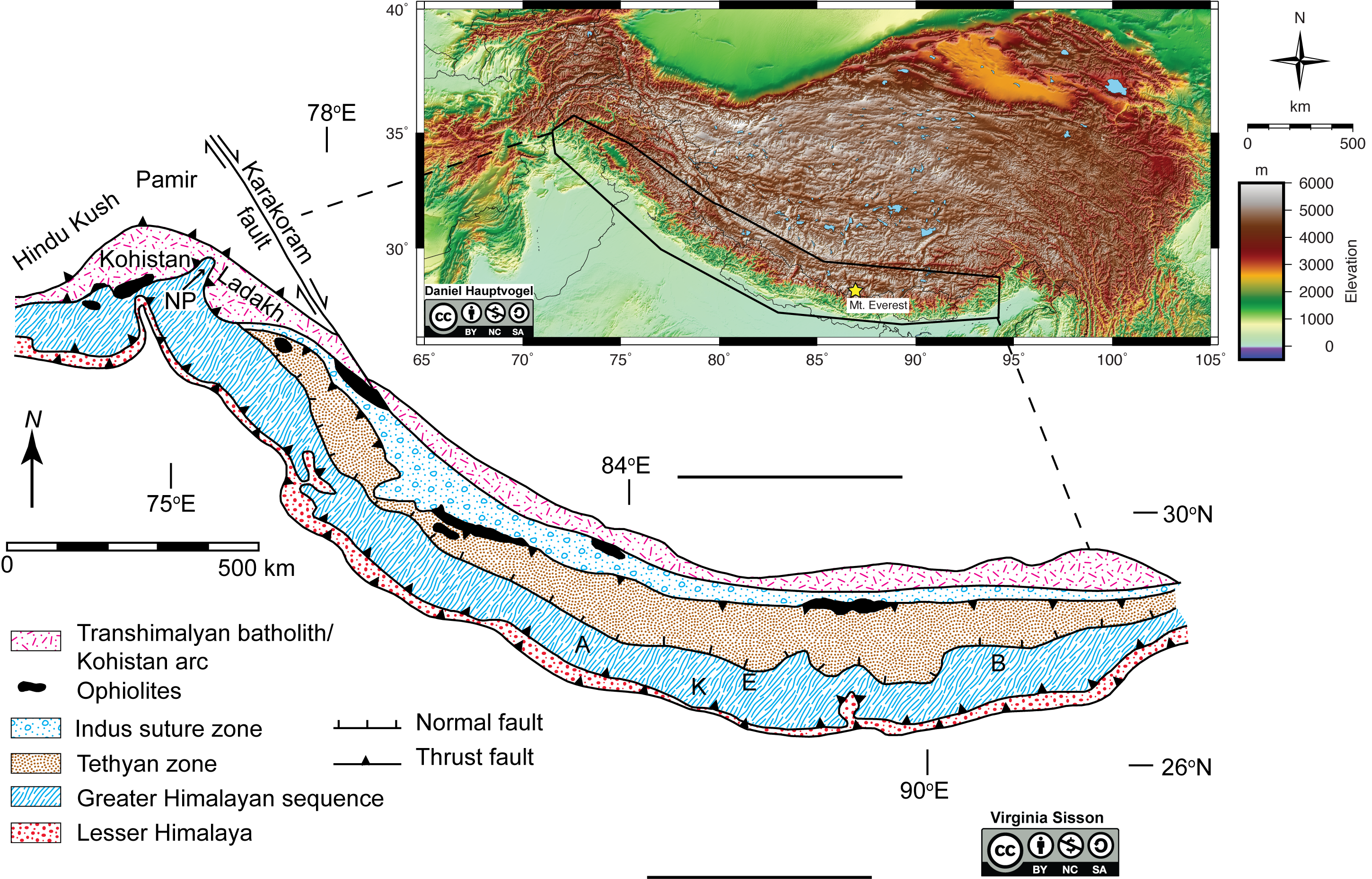
- Now use your knowledge of ophiolites to answer some questions about the geologic history of the Himalayan mountains. In Figure 2.27, name the two tectonic plates. Are these oceanic or continental tectonic plates? What is the thickness of their lithosphere?
- What type of rocks are shown in the black blobs on this geologic map? ____________________
- There are five other groups of rocks in the Himalayan Mountains. Each of these groups has a distinct geologic history.
-
- Why do you think these groups of rocks are distributed as long skinny units?
- If the rock units are elongated in a particular direction, geologists call this their strike direction. Typically strike direction is given as a compass direction. What is the strike direction of these groups? ____________________
- Does the strike change from east to west along the Himalayan Mountains? ____________________
- How does the strike of the ophiolites compare to the contacts between the units and to the thrust and normal faults?
- What can you infer from your observations of the type of faults and the ophiolites? Hint: do the ophiolite blobs occur next to both the thrust and normal faults?
- Why do you think these groups of rocks are distributed as long skinny units?
-
- Make some observations about the map patterns of the ophiolites. Are the ophiolite blobs in a continuous or discontinuous belt?
- Since ophiolites are signatures of previous ocean basins, what happened to all of the oceanic crust that was once between these two continental tectonic plates?
- Critical Thinking: Some geoscientists suggest using the term suture zone to describe where ophiolites occur during continent-continent convergence. Looking at the map, do you think this term is appropriate for the Himalayan Mountains. Explain your answer.
Exercise 2.11 – Southern Alaska
There is a sequence of metamorphic rocks in southern Alaska called the Chugach Metamorphic Complex (Figure 2.28). In one area along the Tana River, you can walk upstream from phyllite to gneiss. However, to determine the metamorphic conditions, you need to identify the mineral assemblages. A team of geologists worked along this river for three summers and mapped the distribution of metamorphic minerals and the deformation, textural, and geochronological history. The outcrops occur where a river along a glacier eroded away the glacial sediments and exposed the bedrock. The protoliths for these rocks are graywacke deposited in an accretionary prism during the Late Cretaceous. Now that you have the geologic history for this region try to interpret the metamorphic pattern shown in Figure 2.28.
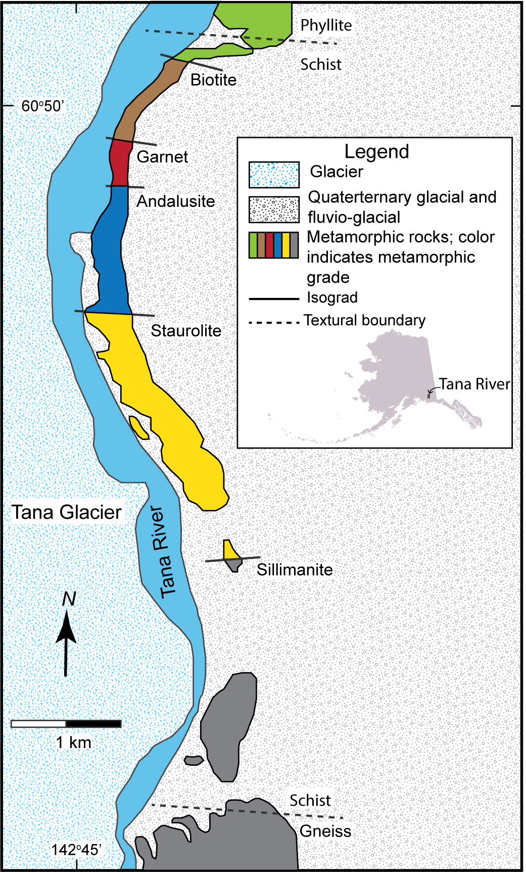
- Do the textural boundaries between phyllite, schist, and gneiss correspond to mineralogical changes? If not, why do you suppose they are different?
- Is this a medium- or low-pressure terrane (consider Figure 2.21)? Did it form as a contact aureole or regional metamorphism?
- Using a graph of metamorphic temperatures in Figure 2.20, what is the difference in temperature from north to south along the Tana River?
- What is the geothermal gradient along the Tana River? To determine the horizontal geothermal gradient, determine the distance between the two points you used for estimating the metamorphic temperature.
- How does the horizontal geothermal gradient compare with vertical geothermal gradients in stable continental crust?
- What was the heat source for the metamorphism?
- Critical Thinking: This map shows the distribution of another mineral common in metamorphosed shales, staurolite. Using the temperature scale, determine the temperature that the staurolite formed.
- Critical Thinking: Assume this area was at ~10 km depth or ~300 MPa. Then, use your temperature estimates from Exercise 2.7f as well as 2.11g to plot the pressure-temperature history for southern Alaska in Figure 2.21. This will be the path that the highest-grade rocks would have taken through time.
Additional Information
Exercise Contributions
Daniel Hauptvogel, Virginia Sisson, Carlos Andrade
References
Berman, R.G., 1991, Thermobarometry using multi-equilibrium calculations; a new technique, with petrological applications, The Canadian Mineralogist, v. 29 (4), p. 833–855
Bowman, J.R., Sisson, V.B., Pavlis, T.L., and Valley, J.W., 2003, Oxygen isotope constraints on fluid infiltration associated with high temperature–low pressure metamorphism (Chugach Metamorphic Complex) within the Eocene southern Alaska fore-arc, in Sisson, V. B., Roeske, S. M., Pavlis, T. P., editors, Geological consequences of ridge-trench interactions in the northern Pacific, Geological Society of America Special Publication no. 371, p. 237-252
Lyubetskaya, T., and Ague, J.J., 2010, Modeling metamorphism in collisional orogens intruded by magmas: I. Thermal evolution: American Journal of Science, v. 310, p. 427-458, DOI: 10.2475/06.2010.02
Pfiffner, O. A., and Gonzalez, L., 2013, Mesozoic–Cenozoic Evolution of the Western Margin of South America: Case Study of the Peruvian Andes, Geosciences 3, no. 2: 262-310, DOI: 10.3390/geosciences3020262
Searle, M.P., and Treloar, P.J., 2019, Introduction to Himamalyan tectonics: a modern synthesis, in Himalayan Tectonics: A modern synthesis ed by P.J. Treloar and M.P. Searle, Geological Society of London Special Publications, v. 483, p. 1-17 https://doi.org/10.1144/SP483-2019-20
Google Earth Locations

a naturally occurring, inorganic, solid that can be defined by a chemical formula and a crystal structure.
a coarse-grained, intrusive igneous rock typically composed of quartz, feldspars, and amphibole/biotite.
a clastic sedimentary rock composed of sand-sized minerals, rock fragments, or organic material
a metamorphic rock made up of bands that differ in color and composition; generally there are light-colored bands rich in feldspar and quartz and dark-colored bands rich in mafic minerals such as biotite or amphibole
how light interacts with the surface of a mineral
color of a mineral in a powdered form
measure of the resistance to scratching by another object or mineral
molten matter beneath or within the Earth's crust from which igneous rocks are formed
an igneous rock that forms when magmas cool beneath the Earth's surface
igneous rocks that form when magma cools at or near the Earth's surface
an igneous rock that is rich in magnesium (ma) and iron (f), often has abundant pyroxene, olivine and amphibole
an igneous rock rich in feldspar (fel) and quartz (si)
sedimentary rocks composed of broken pieces of older rocks
form when minerals in solution become supersaturated and inorganically precipitate
form from the accumulation and lithification of organic matter, such as leaves and other plant or animal material
process where loose grains of sediment are converted into rock, often by cementation
process of transforming clastic sediments into rocks by the precipitation of mineral matter in their pore spaces
a carbonate mineral, CaCO3. This is the stable polymorph at the Earth's surface
mineral consisting of SiO2, silicon dioxide, found in all rock types, the stable polymorph at the Earth's surface
metallic, yellow mineral made of FeS2 and typically occurring as intersecting cubes. Often called Fool's Gold
process in which sedimentary layers are piled up and the sediments beneath are buried, sometimes by hundreds of meters of sediment above
change in temperature with respect to increasing depth. Away from the edges of lithospheric plates, it is about 25–30 °C/km
planar arrangement of structural or textural features in metamorphic rocks along straight or wavy planes
original, unmetamorphosed rock from which a metamorphic rock was formed; sometimes called the parent rock
heterogeneous rock with properties of both igneous and metamorphic rocks; often formed by partial melting
a large mineral in a metamorphic rock which has grown in the fine grained matrix
two or more minerals that have the same chemical composition but differ in their internal atomic arrangement and crystal structure
a series of metamorphic zones with both pressure and temperature increase generally due to continental collision
a sequence of rock layers or formations in the order they were deposited
a representation used to describe the vertical sequence of rock units
a section of oceanic crust and its underlying upper mantle that has been uplifted and exposed, generally now on continental crust
a mass of sedimentary material scraped off of oceanic crust during subduction that piles up at the edge of the overriding plate

_and_quartz_(gray)_grains.jpg#file)