
Chapter 9: Geologic Structures and Mapping
The 2nd edition is now available! Click here.
Learning Objectives
The goals of this chapter are to:
- Visualize geologic structures in maps and cross-sections
- Identify geologic structures on a geologic map
- Learn how to read a geologic map
Some of the maps in this chapter can be printed on poster paper from large PDF files found here (opens in a new tab).
9.1 Introduction
Do you remember in Chapter 0 how we said you would become an expert at reading and interpreting geologic maps? Now is the time to sharpen this skill. In the past, you probably encountered a variety of types of maps. If you have used a mapping app to get directions somewhere, you have used a map. Maps are a scaled, 2-dimensional representation of the surface of an area. Some maps even attempt to portray 3-dimensional landscape features, such as mountains or canyons. This is one of the great difficulties in geology because geologic maps represent 3-dimensional features in a 2-dimensional format. It can be challenging for someone unfamiliar with these features to look at a geologic map and visualize reality. Maps may represent the surface of the land or areas in and around lakes and oceans, the seafloor, or features known or thought to occur underground. Mapping is also used in astronomy (planet and moons, regions of space, etc.). Anything that has a visual distribution can be mapped.
In previous chapters, you have seen how colors and patterns can be used on maps to distinguish different types of rocks, such as volcanic (orangish) versus plutonic (red) in Figure 2.24. Also, the lines between the different colors represent contacts between different rock types.
Before interpreting or preparing a map, it is important to understand some of the background information about the map. Below is a list of information typically associated with maps.
| Information | What it tells you |
|---|---|
| Title | Concise information related to geographic information and map contents |
| Scale | The ratio of distance on the map and distance on the ground. The scale should be relative to both kilometers and miles. Most maps also have a visual scale bar of relative distance on the map. |
| Orientation | An arrow pointing north and, if possible, latitude and longitude |
| Explanation or Legend | Explanation of any symbols used on the map, including colors, lines, or icons. |
| Reference features | Selected reference locations or features such as a town, river, state boundary, mountain, etc. |
| Source information | A list of authors, compilers, editors, publishers, associated publications (text or guidebook), URL, and any other information so it can be accurately cited in reference list or bibliography. |
| Base map information | What is the source of the geographic information? For example, is it based on a USGS topographic map, or is it a satellite image? What is the map projection? |
| Date published | The year the map was released or revised. |
| Written text | Is there a publication or guidebook associated with this map? |
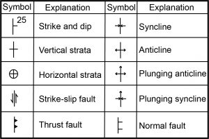
What do you need to know for geologic maps? First, there are lots of standard symbols used to help geologists worldwide use the same terminology. You also need to be able to read strike and dip symbols. If you didn’t learn about strike and dip in Physical Geology, now is the time to do so. Most geologic maps will have a stratigraphic column with either colors or patterns to distinguish various rock units. Again, there are often standard colors for different ages of rocks and patterns for the rock types. Look at the tables in Chapter 2 Earth Materials to see some common patterns for different rock lithologies. Figure 9.1 shows the common symbols used for geologic structures.
Exercise 9.1 – Mississippi River Maps
The Mississippi River has evolved throughout its history as the river channel has meandered back and forth across the landscape of the central U.S. Different types of maps can provide some insight about previous river channels and how we can distinguish them. What you learn from the Mississippi River will help you understand river systems throughout the world, regardless of their size.
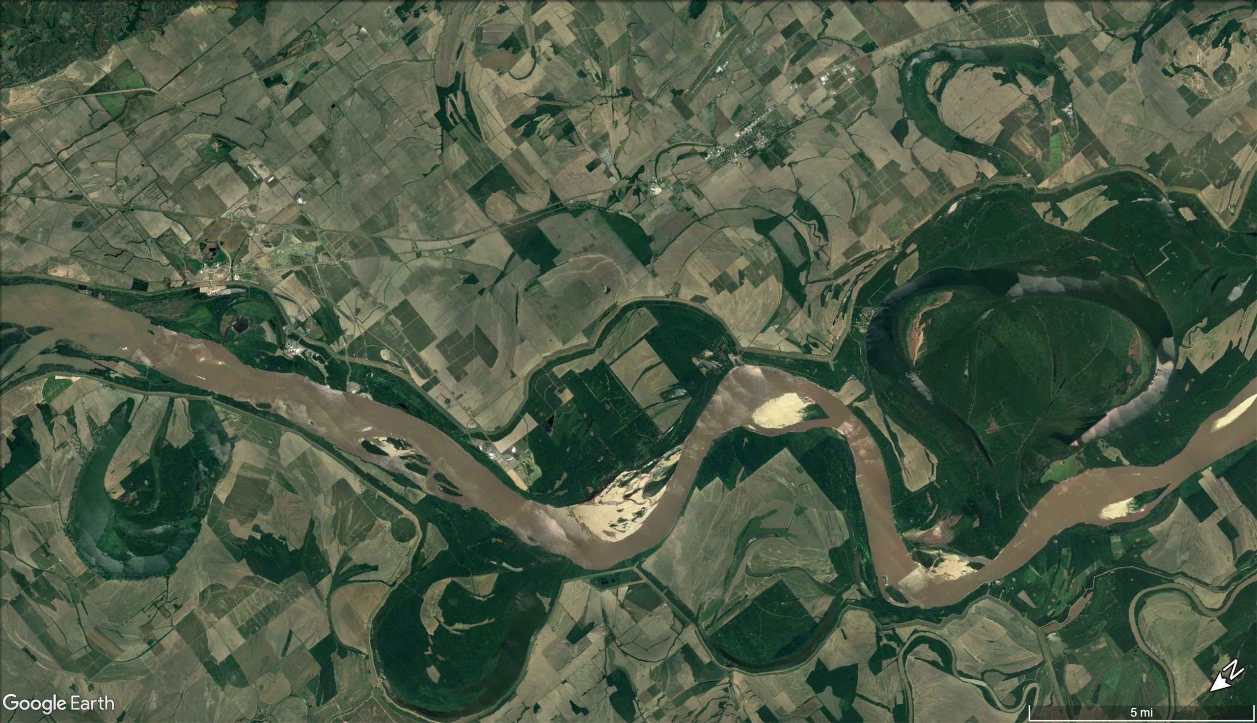
Part 1: Aerial Imagery
Figure 9.1 is a satellite photograph from a section of the Mississippi River from Google Earth. Think of this image as what the ground looks like from an airplane. You can see vegetation that has responded to the river evolving and patterns associated with the river.
- Trace three previous paths the Mississippi River has taken. It is ok if these channels cross where the river is currently. Label the different paths a, b, and c, and use color to differentiate them.
- Put the paths that you identified in order from the most recent to the oldest. ____________________
- What is your evidence for this order?
- What is your evidence for this order?
- Locate and mark at least five features associated with a river system. Examples could include cut bank, point bar, levee, oxbow lake, thalweg, flood plain, terrace, etc.
- What are some of the difficulties you experienced with completing these two questions?
- How do you think we could solve some of these problems? What data would you need to accurately assess the true paths and their ages?
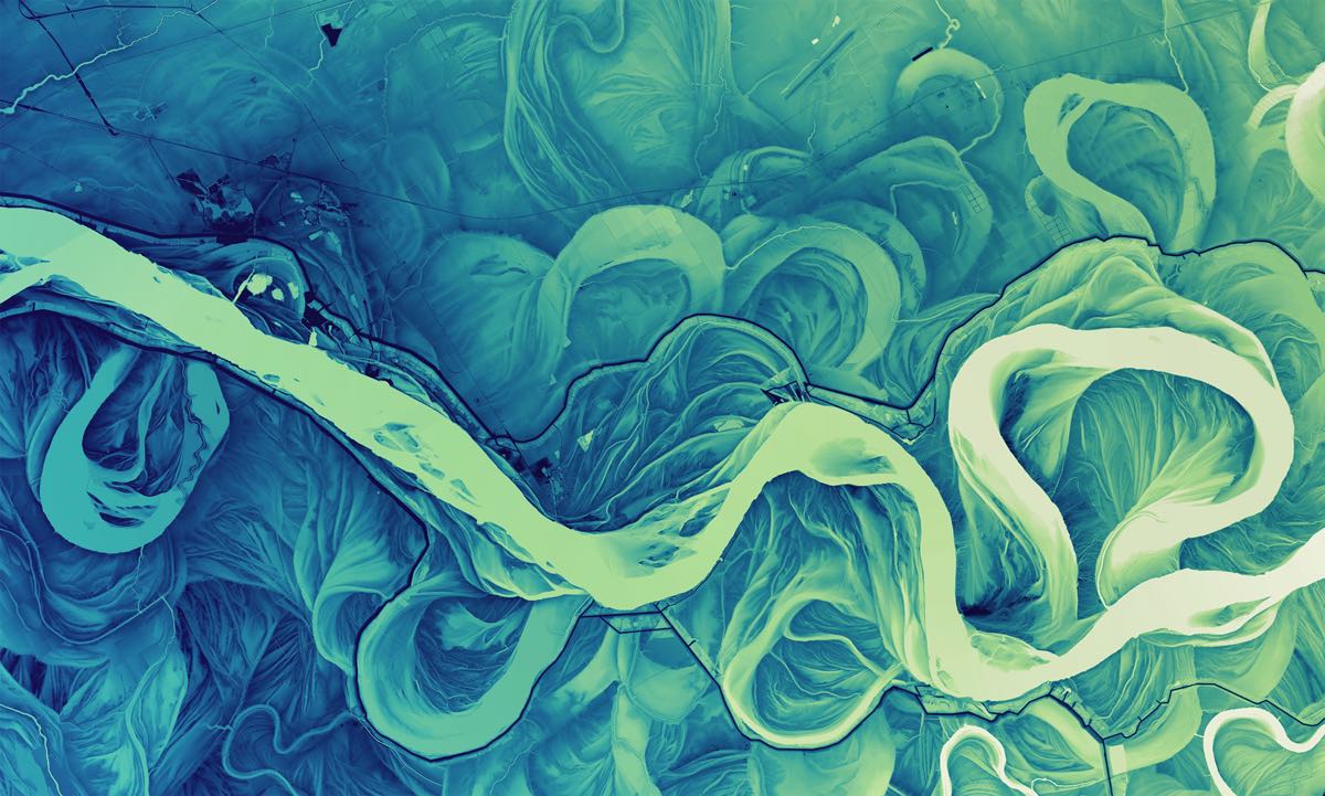
Part 2: LiDAR Imagery
Look at the second image (Figure 9.2). This image was made by using LiDAR. This method uses wavelength reflections to produce detailed images of topography. Different wavelengths are susceptible to changes in interference and reflection caused by vegetation and sediment changes, which can help identify previous channels.
- See if you can locate the channels you found in Part 1. Explain why you agree or disagree with the locations you placed previous river channels?
- In Figure 9.2, locate and mark three previous paths the Mississippi has taken that are different from those you identified from Figure 9.1. Label them with d, e, and f.
- Using your three paths from Part 1, and your three paths from this part, try to place the six channels in order from the most recent to the oldest. ________________________
- What are some of the problems you are encountering doing this?
- What are some of the problems you are encountering doing this?
- Explain how this image helped or didn’t help you identify the proper paths the Mississippi River has taken.
- Do you think it is necessary to obtain more data to solve our problem of finding previous paths and ages?
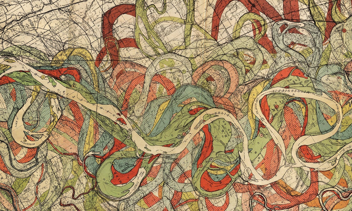
Part 3: Geologic Map
Figure 9.3 is a map of previous river paths the Mississippi has taken. It was made by a geologist before the ability to use Google Earth or LiDAR images.
- Locate as many paths as you can that you have identified from the previous images. Do you still agree with where you placed the channels you found? Why/why not? Keep in mind that just because a geologist made this map, it may not be 100% correct.
- See if you can put the paths you’ve identified from the previous images in order from most recent to the oldest. Explain if you were able to identify a different order, add more paths you hadn’t seen before, or if you notice anything else that you think is important.
- How has this image helped in understanding the proper paths the Mississippi River has taken? Do you think it is necessary to obtain more data, such as drill cores, to solve our problem of finding previous paths and ages for analysis? Explain.
- Critical Thinking: Where would you put a drill core? Explain.
- Critical Thinking: Could you describe how and where the river moved from its creation to now in such a manner that someone could draw snapshots in time? Try it.
9.2 Geologic Structures
You already know that the Earth is a dynamic place and that plate tectonic forces bend and break rocks. You’ve already studied this subject in both Physical Geology text and lab books. Here is a short review of some of the concepts you will need for this chapter and the next. Some students have an easy time visualizing in three dimensions. If you have trouble with this, practice with block diagrams.
Remember those lab exercises on geologic time and stratigraphy? While doing these, you looked at vertical sections and views of cliffs, but now you need to be able to decipher geologic patterns on maps. If you need a refresher or perhaps a glimpse of geologic maps with different map patterns, check out these links to flat stratigraphy in Nebraska, three types of unconformities in Saskatchewan, thrust fault in the Olympic Peninsula, plunging anticline in Wyoming, plunging anticlines and synclines, normal faults (core complex in Arizona), and a strike-slip fault in New Zealand.
Strike and Dip
When deformation occurs, sedimentary layers are no longer flat-lying and instead lie at an angle. This angle is called the dip (Figure 9.5). The dip is a measure of the steepest possible slope, sometimes referred to as inclination. You can imagine water running down the surface; it will take the steepest path in the dip direction. It is common for geologists to pour a little water on a rock surface to see how the water runs, telling them the dip direction. The strike of a plane is a bit more complicated. Strike is the horizontal line that forms as a dipping bed intersects with the surface (Figure 9.5) and is always 90° from the dip direction. Geologists measure the orientations of geologic features using a Brunton Compass, a special compass that has a set of levels to take accurate measurements of features. To determine the orientation of these dipping bedding planes, you need to measure both strike and dip.
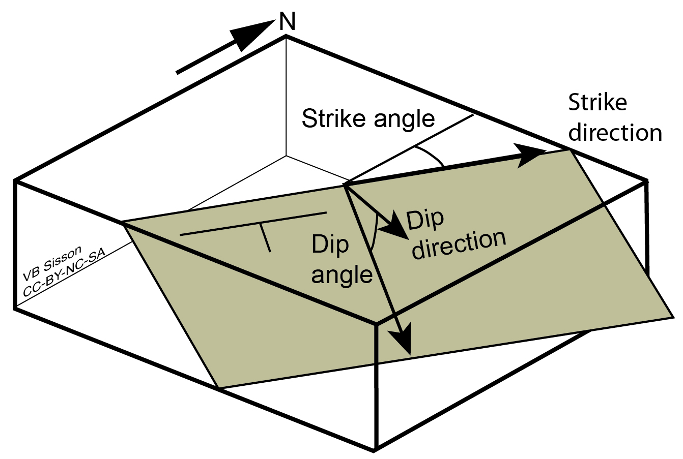
There are two directions you can measure the strike that are 180° apart. The dip direction is clockwise from one and counterclockwise from the other. In most geological fieldwork, the right-hand rule is used. If you place your right hand on the dipping layer with your fingers pointed toward the dip, then your thumb is pointing in the strike direction. In other words, the strike is always 90° counterclockwise from the dip direction.
When writing out the strike and dip, it is a good idea to add the compass direction to the dip measurement, just as a check that you’ve done the right-hand rule measurement correctly. For example, in Figure 9.5, the strike is 40°, and the dip of the plane is 30°, so this would be written as 040/30 SE. This is a plane that dips at 30° with strike roughly NE. The dip direction is clockwise from the strike, so the dip direction is SE. You can check this since 225/30 would dip to the NW to follow the right-hand rule, not the NE.
Anticlines and Synclines
Folds are some of the most dramatic geologic structures. These form when the Earth’s crust is shortened during compression associated with plate tectonic convergence. Folds are important economically as many resources accumulate in the folds, such as petroleum or gold in anticlines. The points of the tightest curvature are called the hinge. In contrast, the limbs are the areas of least curvature. If the limbs dip away from the hinge, this is called an antiform. If the limbs dip toward the hinge, this is called a synform. Note that if the fold closes on its side, it is impossible to tell if it is an antiform or synform.
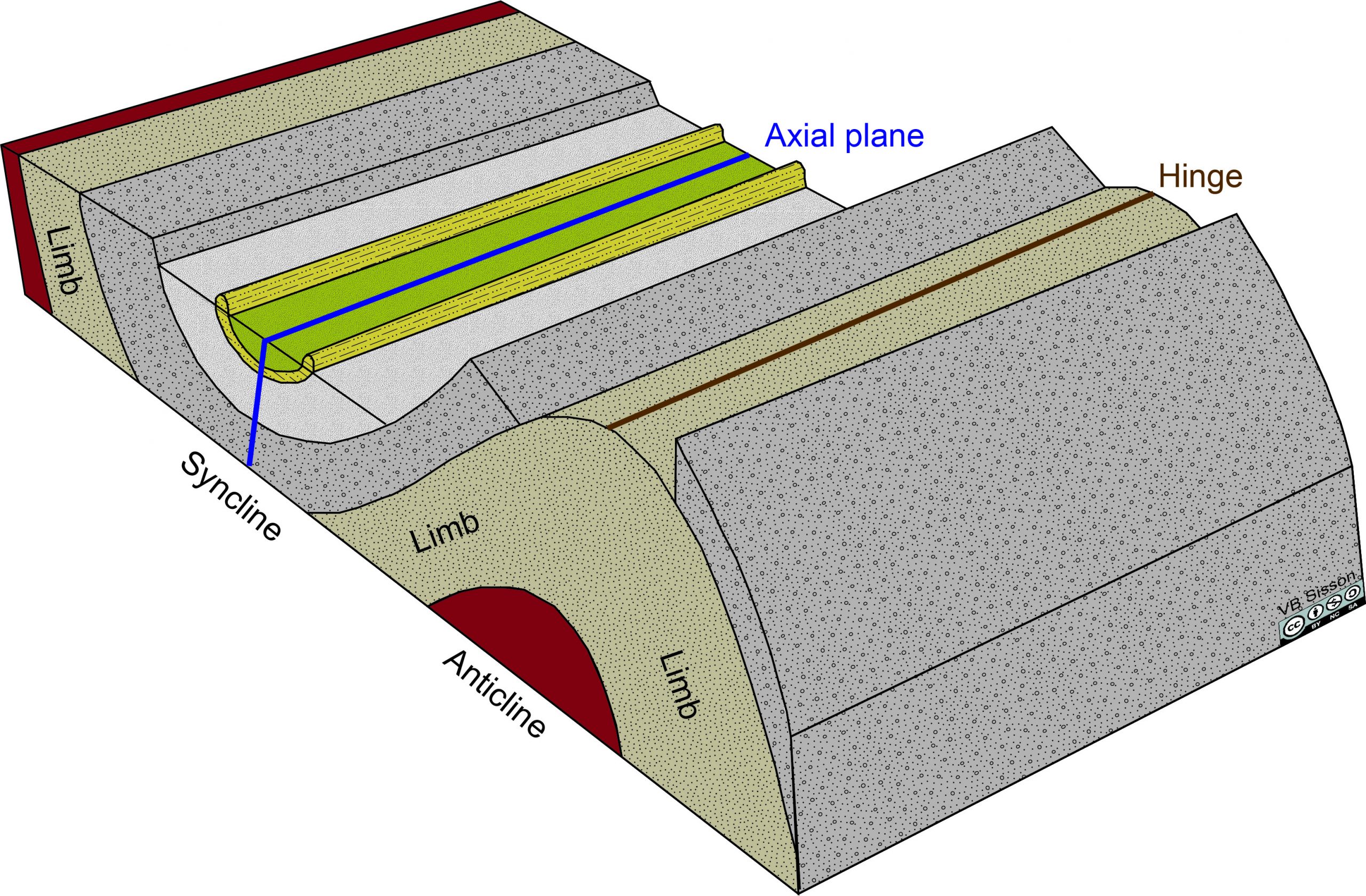
In a stratigraphic sequence of folded sedimentary rocks, the rocks get younger towards the inside of a syncline and older toward the inside of an anticline, then the fold is a syncline.
The hinges of folds can be connected to create an axial line. If this line is horizontal, the fold is non-plunging. However, if the axial line is tilted, then this is a plunging fold.
If you draw a plane connecting all of the hinges or axial lines of each sedimentary layer in a fold, this plane defines an axial plane. This can be oriented vertically, be inclined, or even flat-lying or horizontal. If the axial plane is horizontal, the fold is classified as recumbent. The dip of the axial plane can be used to classify the type of fold (Table 9.2).
| Dip | Fold Type |
|---|---|
| 0-10° | Recumbent |
| 10-30° | Gently inclined |
| 30-60° | Moderately inclined |
| 60-80° | Steeply inclined |
| 80-90° | Upright |
Faults
Faults are fractures through rocks that have had a significant amount of movement on them. Strictly speaking, a fault is a single brittle fracture, whereas a fault zone has multiple brittle fractures, and a shear zone is a ductile fault (Figure 9.7).
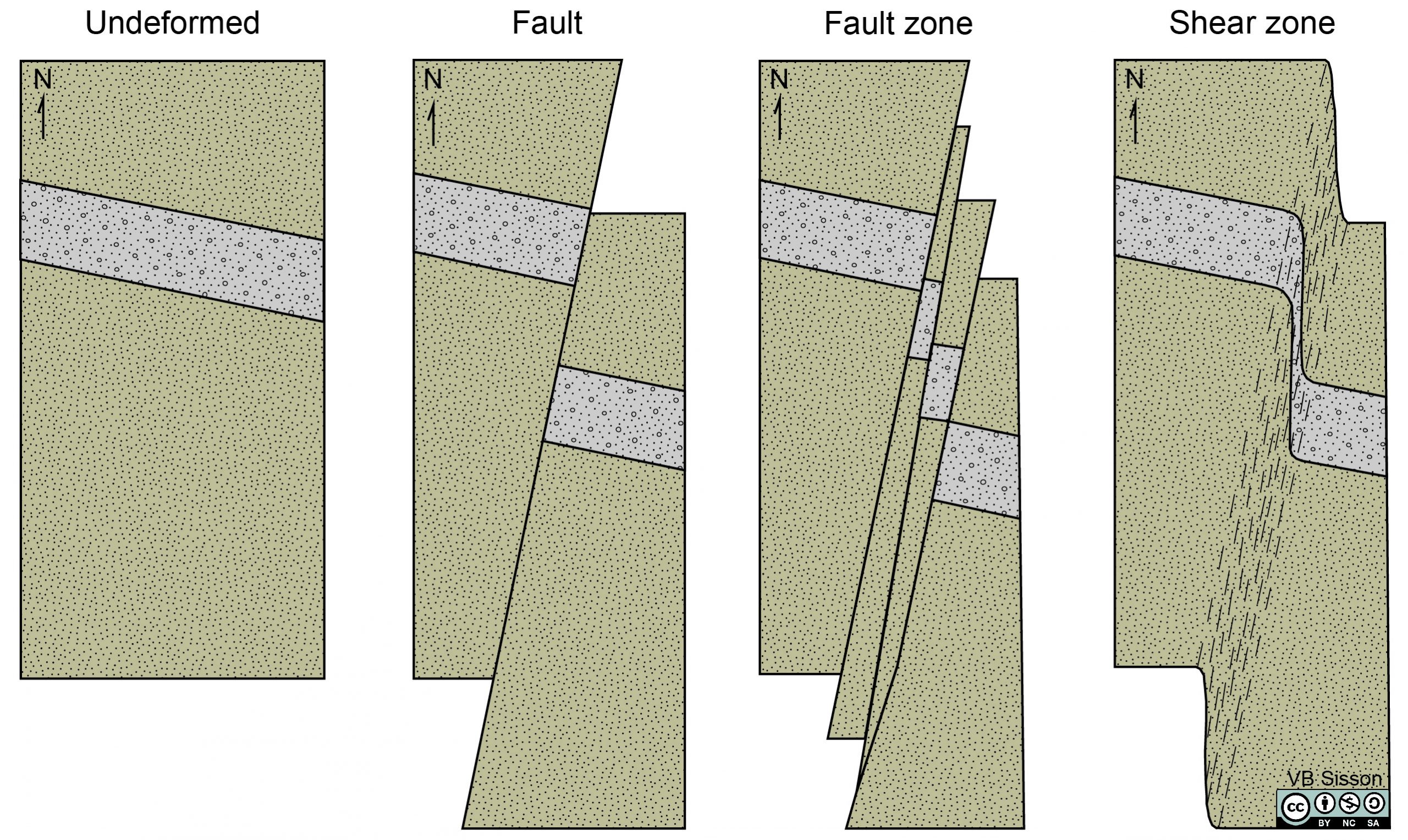
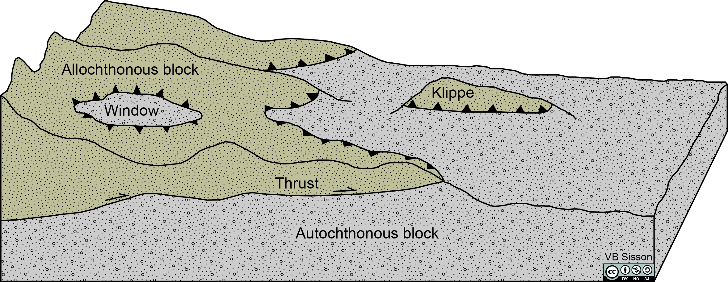
The blocks on either side of a fault are called the walls. If the fault has a vertical orientation, this is a strike-slip fault with horizontal displacement. If the fault has a dip that is not vertical, then one wall is over the other with dip-slip motion. The blocks are defined as either the footwall or hanging wall. There are two types of faults with dip-slip motion: normal faults formed during extension and reverse faults formed during compression and shortening of the Earth. In normal faults, the hanging wall moves down. In reverse faults, the hanging wall moves upwards. There is a special type of reverse fault with a gentle fault that dips less than 30°, called a thrust fault, which is more common than reverse faults (Figure 9.8). For thrust faults, the block that moves is called the allochthonous block that is thrust over the autochthonous block. Erosion may isolate some of the allochthonous block as a klippe. It may also expose the autochthonous material in a window.
9.3 Geologic Maps
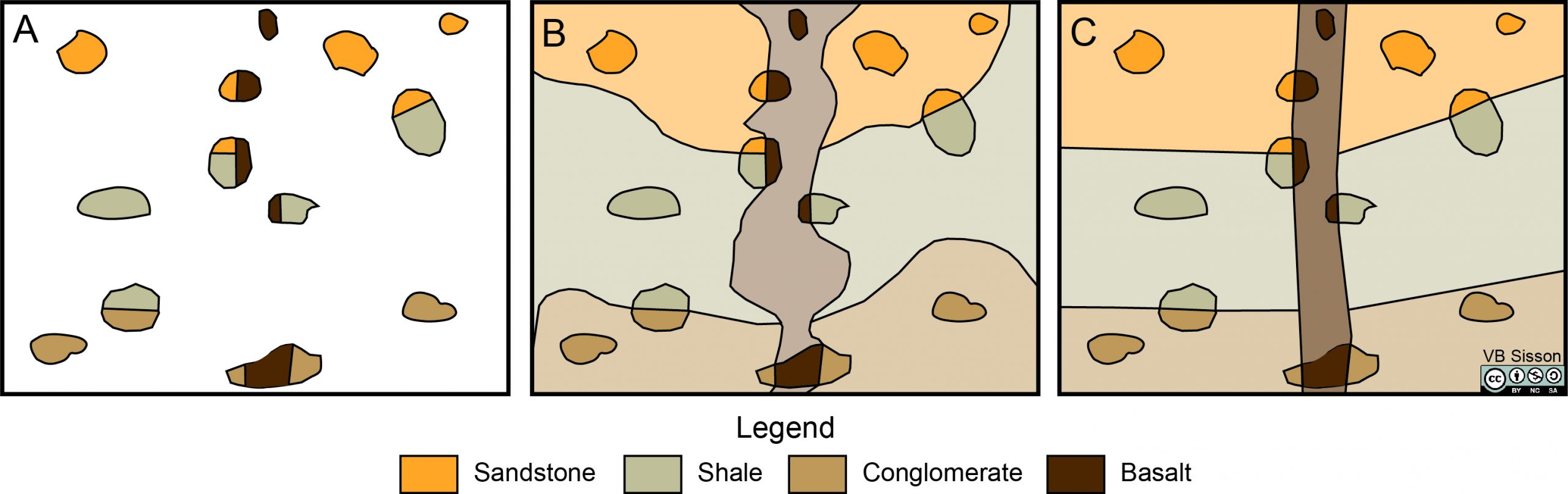
To make a geologic map, you need to use your geological skills to fill in the areas between data points, such as outcrops, stratigraphic sections, wells, soil profiles, etc. Often the data is imperfect and doesn’t cover 100% of the area in question. For example, figure 9.9 shows an outcrop map and two possible attempts at geological maps. One is made without much understanding of geological processes. Although it satisfies the observations in a simplistic way, it is unlikely to be correct. The other attempt is a more likely interpretation made with some understanding of geological processes. In this case, there are three sedimentary units; these probably have parallel boundaries. Also, there is a basalt which you can see from some of the outcrops that is probably a dike that cross-cuts the sedimentary layers. So, to interpret this outcrop pattern, you have to use your knowledge of sedimentary contacts (Chapter 4) and cross-cutting relationships of basalt dikes since you know that they are often straight (Chapter 3).
Do you remember the rule of V’s for maps? There are two different versions of this rule; one for topographic maps and the other for geological maps. If you see a V shape in a topographic map, then the point of the V points upstream toward the source. In geological maps, this rule governs the intersection of the geologic features, such as dikes, sills, faults, bedding planes, fold hinges, etc. with topography. The easiest two features to remember this is that horizontal features such as sedimentary layers and sills will be parallel to topography, whereas vertical features such as dikes will cross-cut topography (Figure 9.10). You can use the angle of V formed by the intersection of a linear feature and the topography can help you determine the dip of the feature. If you need help seeing these relationships in three dimensions, look at these models.
Cross-sections
You learned how to make topographic profiles and cross-sections in Physical Geology. You may want to review how to do this before starting the exercises. Remember that vertical scale is one of the features in a cross-section, and it may not be the same as the horizontal scale. If these are the same, there is no vertical exaggeration. In many cross-sections, the horizontal scale is longer than the vertical scale. This is common in many seismic reflection profiles. This may exaggerate sedimentary layer thickness as well as the dip of some features. In general, the apparent angle of dip increases with increased vertical exaggeration. For example, for a thrust fault dipping at ~25o, it will appear to dip 60o with ~3x vertical exaggeration. This will make it difficult to differentiate a thrust fault from a reverse fault in your cross-section. So, it is important to include the vertical exaggeration for any of the cross-sections you create while interpreting geologic maps.
An important feature on cross-sections is the dip of any contacts, which can range from flat to vertical. If the cross-section is constructed perpendicular to the strike of dipping layers or contacts, then the cross-section will show the true dip of the features. If the cross-section is not perpendicular to the features, the apparent dip of the layers will be less than the true dip.
Another way to visualize cross-sections through an area is to construct slices through a three-dimensional (3D) seismic survey. You may think this is a new technology, but the first 3D survey was made by Exxon across the Friendswood oil field near Houston, Texas, in 1967. For a 3D seismic survey, seismic data is acquired along closely spaced parallel lines that are processed and interpreted as a volume of data. Modern 3D surveys have seismic traces spaced at ~12.5 meters. These seismic volumes are also called seismic cubes.
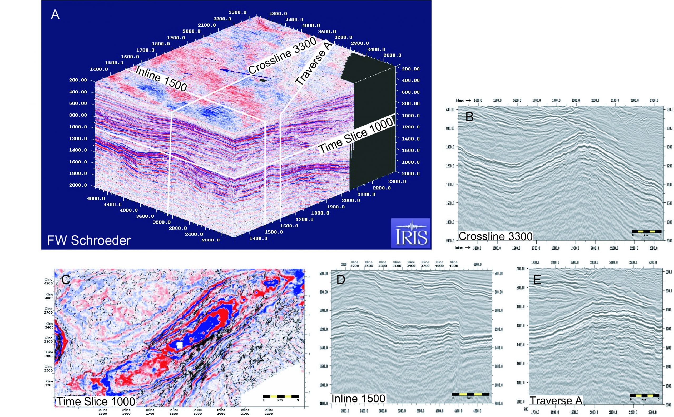
Figure 9.11 shows a 3D seismic cube through a folded sequence of sedimentary rocks and several two-dimensional cuts through this cube. Cross-sections through the 3D seismic cube are identified relative to the direction that the seismic survey was shot. A cross-section parallel to the direction of the survey is an inline view. A cross-section that is perpendicular to the survey is a crossline. You can also slice horizontally through the seismic cube and create a time slice. Finally, you can make an arbitrary traverse to better show structural features.
Exercise 9.2 – Create a Simple Geologic Map and Cross-Section
Your instructor has placed model stations around the classroom. You need to note lithology and collect structural data from each model station. Go around the lab room using the Clino app (free from the Apple app store and Google play store) to measure the strike and dip of the model outcrops and make color-coded notes of their lithology.
- Make a geologic map using the data points collected from the outcrops you visited in this exercise. Make sure to use appropriate colors for the rock units and appropriate structural notation. Remember that your map should have a scale and a north arrow. Draw contacts between the different rock types. At each station, you should put a strike and dip symbol using the right-hand rule.
| Geologic Map: |
- Make a straight line that crosses the contact lines in your map. If possible, the cross-section should be perpendicular to your contacts. This line will be where you construct a cross-section of your map. Label the two ends of the cross-section. Typically cross-sections are labeled as A-A’ or A-B. Show the location of your cross-section on your geologic map. Remember that since the desks are flat in the lab, you don’t need to worry about the topographic profile for this cross-section. Did you use any vertical exaggeration for your cross-section?
| Cross-section: |
- Critical Thinking: Imagine you found some fossils in these sedimentary units. Remember your laws of superposition and add into your cross-section which layer would have a Paradoxides trilobite and which would have a Mucrospirifer brachiopod.
Exercise 9.3 – Using Google Earth to Interpret Geologic Structures
Head to this Google Earth tour to look at geologic structures in Morocco, a country in northwestern Africa that borders the Atlantic Ocean and the Mediterranean Sea. Morocco is currently part of a passive margin but historically was tectonically active. The geologic history of Morocco started about two billion years ago, in the Paleoproterozoic with the Pan-African orogeny. Then, another tectonic event involved the collision of Euramerica (or Laurussia) with Gondwana during the Hercynian orogeny (in eastern North America, this is the Appalachian orogeny). During the Paleozoic, extensive sedimentary deposits preserved marine fossils. Throughout the Mesozoic, rifting broke up Pangaea forming the Atlantic Ocean. These basins and fault blocks were blanketed in terrestrial and marine sediments. In the Cenozoic, a microcontinent covered in sedimentary rocks from the Triassic and Cretaceous collided with northern Morocco, forming the Rif region. Morocco has extensive phosphate and salt reserves, as well as resources such as lead, zinc, copper, and silver. Morocco is also a fossil hunter’s paradise with exquisite trilobites and ammonites.
- What geologic evidence would you look for to see if an area was tectonically active in the past?
Overview
Start the tour and look at the Overview stop. This is the first geologic structure we will look at
- From this aerial view, how would you describe the appearance of this structure?
- Do you think this structure is made of igneous, sedimentary, or metamorphic rocks? ____________________
- Trace three layers as far as you can on the tour screenshot in Figure 9.12
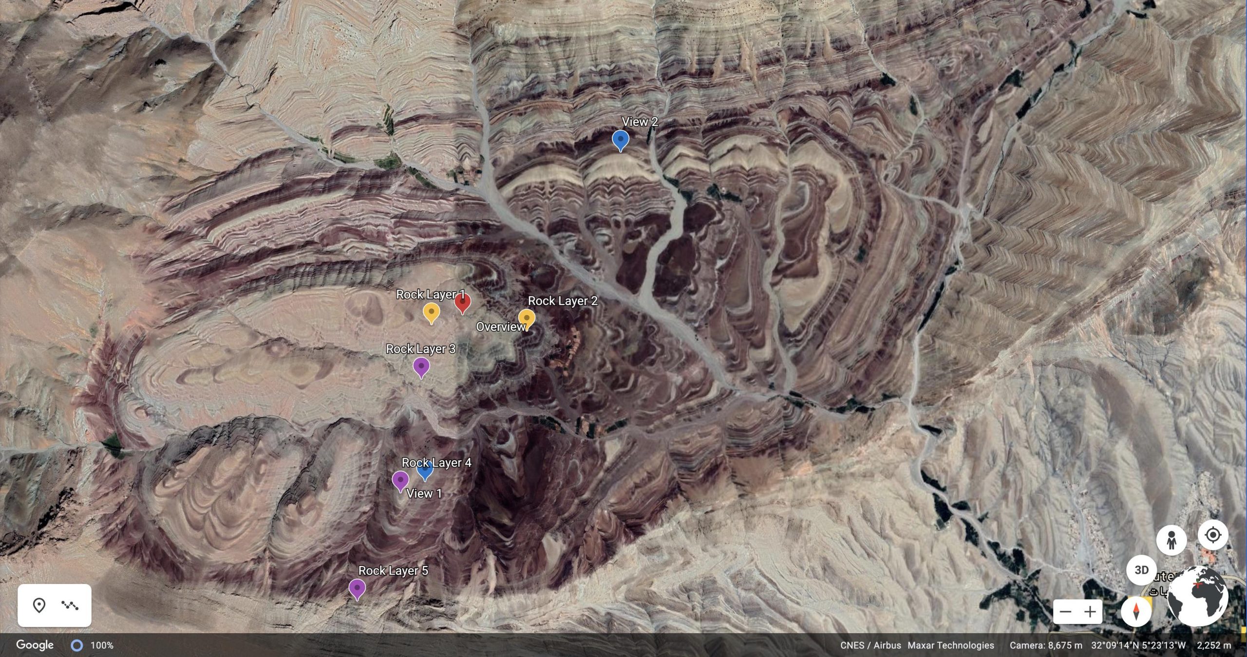
Views 1 & 2
- Look at View 1. Are the layers of rock horizontal or tilted? _______________
- If the layers are titled, in what direction are they dipping toward. (HINT: the red triangle on the compass on the bottom-right always points north.) _______________
- Look at View 2. Are the layers of rock horizontal or tilted? _______________
- If the layers are titled, in what direction are they dipping toward. _______________
- What geologic structure are you looking at? _______________
- Look at Rock Layer 1 and Rock Layer 2. Determine and explain which one is older.
- Look at Rock Layers 3, 4, and 5. What is the age relationship between these layers?
- Explore the map. Locate similar structures.
Geologic Map and Cross-Section
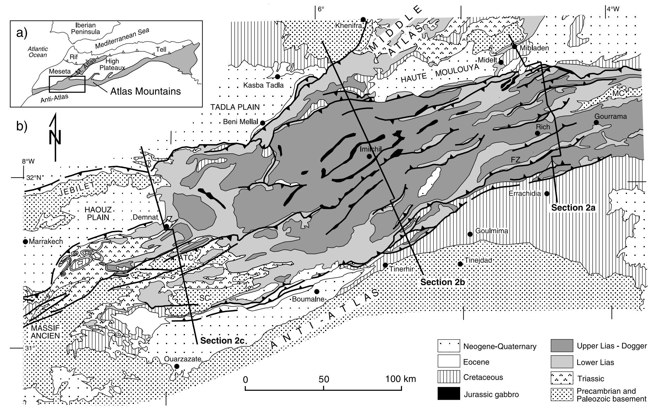
Figure 9.13 is a geologic map of the region. The location of the structure is right near the town of Imilchil, toward the center of the map. Figure 9.10 is a cross-section along the line labeled Section 2b. There are a couple of items that you need to know to be able to read this map and cross-section. First is that this region was originally mapped by French geologists. So, they used European names for geologic time such as Lias and Dogger. Secondly, a shallow basin formed during Triassic rifting of Pangea; these sediments include salt and red beds (hematite-rich sediments). After the basin filled this salt rose, forming diapirs and pillars in a wide variety of shapes. Subsequently, the area was deformed by folding and thrusting during the continental collision between the African and European plates.
- What is the age of the predominate sedimentary rocks exposed along section 2b? _______________
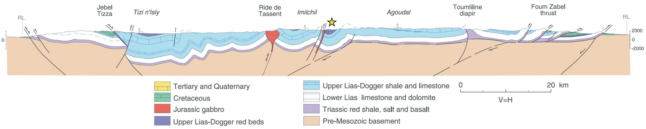
- Find three different sedimentary units, following them across the cross-section. Which unit is the most continuous? Which unit is the least continuous?
- Is there evidence of an unconformity? If there is, mark on the cross-section where it is. Identify the type of unconformity.
- On the cross-section, label the anticlines and synclines.
- Label and identify which kind of faults are present in this area.
- What type of structure formed the Toumliline diapir?
- Give a generalized geologic history with the relative stratigraphic, igneous, and deformation events.
The Grand Canyon and adjacent U.S. National Parks cover the entire stratigraphic section from Early Proterozoic to Holocene. This sequence records almost continuous sedimentation with gaps in time (unconformities). This entire section is not exposed in one National Park. In addition to having an awesome exposure of sedimentary rocks, the area has also undergone deformation with faults and folds; this occurred between 70 and 30 Ma ending with the uplift of the Colorado Plateau. If you want to keep track, there are ~40 major sedimentary units in the Grand Canyon.
Exercise 9.4 – Grand Canyon
One of the most complete records of geologic time is in the Grand Canyon. So, this is an excellent area to learn how to read geologic maps. Before beginning this exercise about the Grand Canyon, you should review the stratigraphic section in Figure 2.25 or look at the sketch by Powell in Figure 0.3.
Getting the Map
If your department has a poster printer, you can print out a large version of the geologic map of the Grand Canyon from this file (opens in a new window). This map is from a USGS poster, but we have removed much of the extra material. Otherwise, you can use this interactive online version of the map.
For fun, you want to look at a 3D geologic map. Another way to look at the Grand Canyon is to use Google Streetview. Start at the South Rim on this map, and drag the orange person icon onto one of the trails to view the rocks from inside the canyon! Or, if you want to do more, you can look at an immersive virtual field trip to see more of the canyon for yourself!
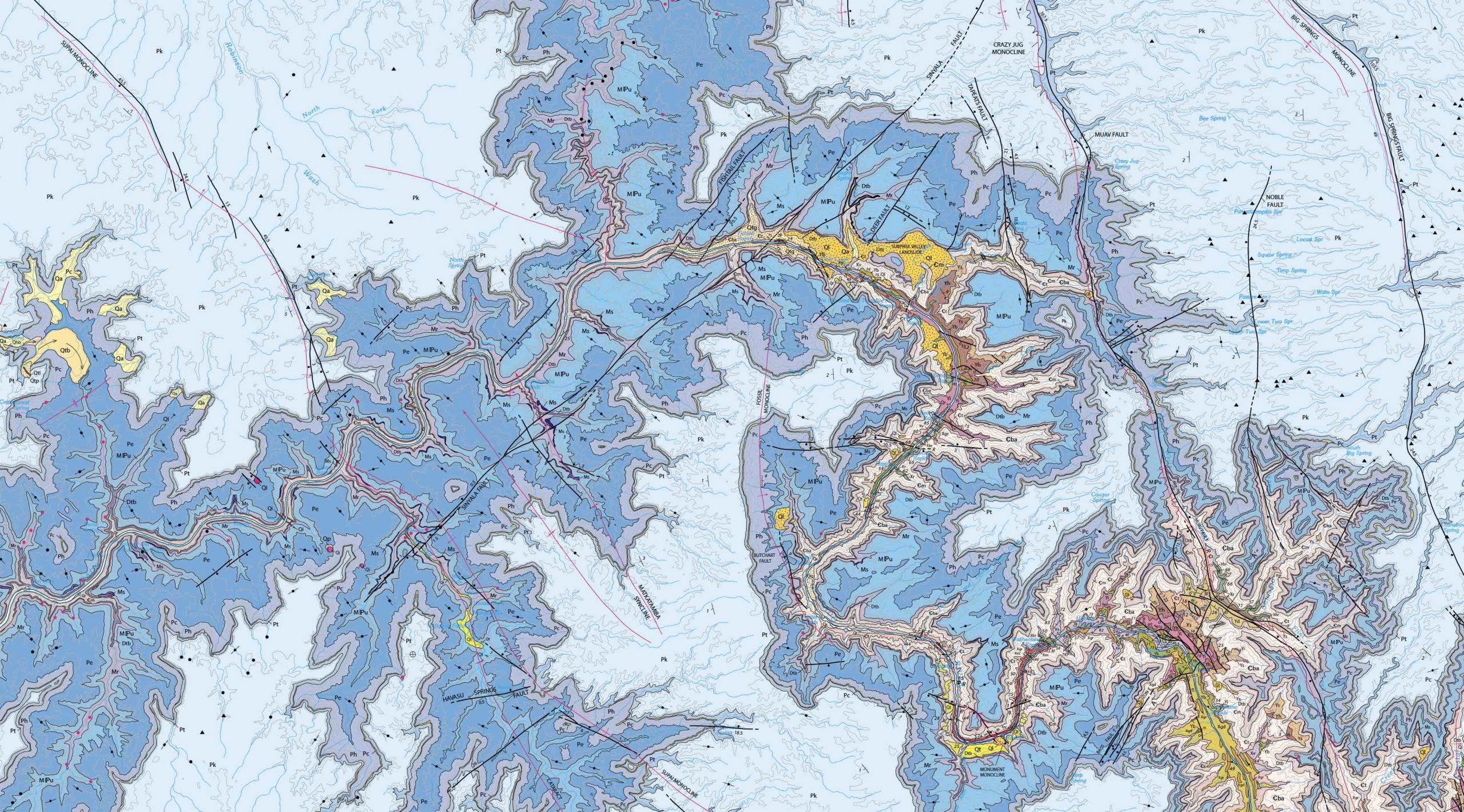
Part 1: Map Reading
- What is the dominant rock type in this map? ______________________________
- What is the age of about 80% of this map? Give its geologic period. ______________________________
- Find an example of each type of structure including three types of folds, two types of faults, dipping and horizontal beds, sinkhole, collapse structure, and pyroclastic cones.
- Which stratigraphic unit is the oldest? Which is the youngest? Give their geologic period and name. ______________________________
Part 2: Timing
- Locate on the map the Great Unconformity and estimate its time gap. _______________________________________
- On the map, locate the Greatest Unconformity and estimate its time gap. _________________________________
- Which of these has the greatest time gap?____________________________
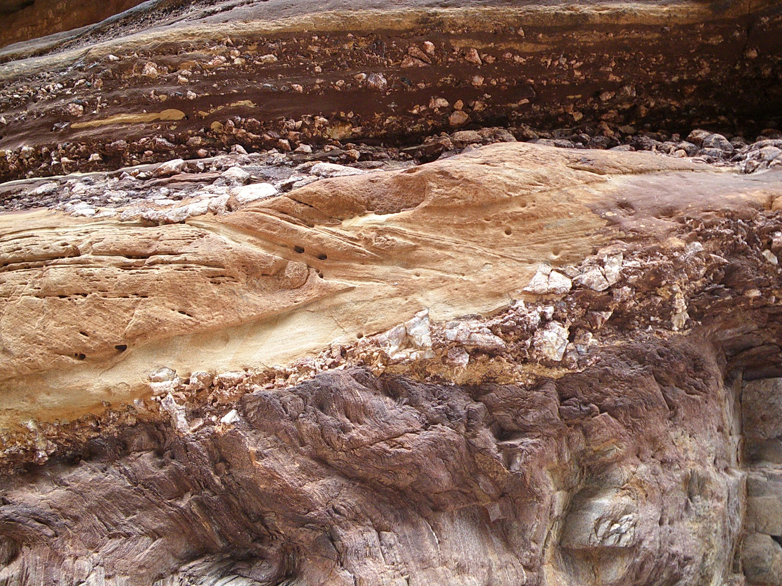
- Critical Thinking: The Great Unconformity is an iconic geologic feature that marks the boundary between non-fossil-bearing Precambrian rocks and fossiliferous Phanerozoic strata. In North America, it spans from Mexico to Canada. Can you explain why there is this unconformity? What would you look for in either the map pattern or an outcrop (Figure 9.16) to support your hypothesis?
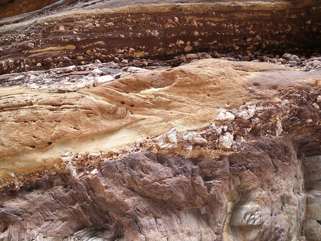
Figure 9.16 – The Great Unconformity in the Grand Canyon with Vishnu schist overlain by Tapeats sandstone. Image credit: Al_HikesAZ CC BY-NC 2.0.
Part 3: Map Patterns
- Describe or sketch the map pattern for a nonconformity.
- Describe or sketch the map pattern for an angular unconformity?
- Using the Rule of V’s, describe or sketch the map pattern for flat-lying sedimentary units.
- Critical Thinking: Can you tell from the map pattern which is a resistant rock unit?
Part 4: Critical Thinking about the Geologic History
- What is the age of the Bright Angel fault? _______________________________
- There are a series of parallel faults such as the De Motte and Uncle Jim Faults. Using Rule of Vs and their map pattern, are these vertical, horizontal or dipping faults? ____________________________________________________________________________
- Is the Kaibab anticline older or younger than these faults? Explain.
- Some think the Grand Canyon started to form only 5 million years ago when the Colorado River started to cut through the stratigraphy. Others say the Grand Canyon started to form in the Laramide 50 to 70 million years ago. Are there any features on this map that support either hypothesis? Look at the ages of the rocks and faults that are cross-cut by the Colorado River to support your answer.
- Critical Thinking: Using this map, construct a geologic history beginning in the Cambrian and ending in the Holocene. Here is a youtube video of past plate configurations. Anytime the area is blue, it was underwater. Green and brown indicate was landscape and subject to erosion and/ or tectonic uplift.
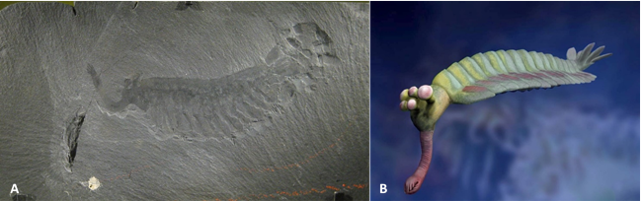
The Burgess Shale in Yoho National Park in British Columbia, Canada, is a world-famous fossil locality. This locality is famous for its 508 Ma fossils that mark the Cambrian explosion. These are one of the earliest fossil beds that contain soft-bodied imprints of a wide variety of life forms. Many of these are ancestors of higher life forms such as chordates, while others appear unrelated to any living forms. Charles Walcott, Secretary of the Smithsonian Institution, first discovered these in 1909. Walcott collected over 65,000 specimens. Nearby there are other quarries that are still yielding new specimens. There are over seventy similar localities for soft-bodied Cambrian fossils! They were initially described in Vermont 25 years before the Burgess Shale discovery.
One example of a bizarre animal from this location is Opabinia which had five eyes, a backward-facing mouth as well as a proboscis to scoop out prey from the marine muds. Only twenty specimens of this animal have ever been described; they all come from one layer within the Walcott quarry site. No one agrees on what family this carnivore belongs to; some say primitive arthropods and others trilobitoids.
Exercise 9.5 – Burgess Shale
Before you begin to look at the next map, it is useful to remember some of the principles of using a topographic map that you learned in Physical Geology. In this exercise as you’ll be using a Canadian map, which uses different scales compared to maps from the U.S. Geological Survey. So, the contour intervals will be different as well as its scale. Contour intervals generally are inversely proportional to the map scale and also depend on whether the area has flat or steep topography. So, by just determining this, you’ll be able to judge whether or not you’ll be able to easily hike through the area or not.
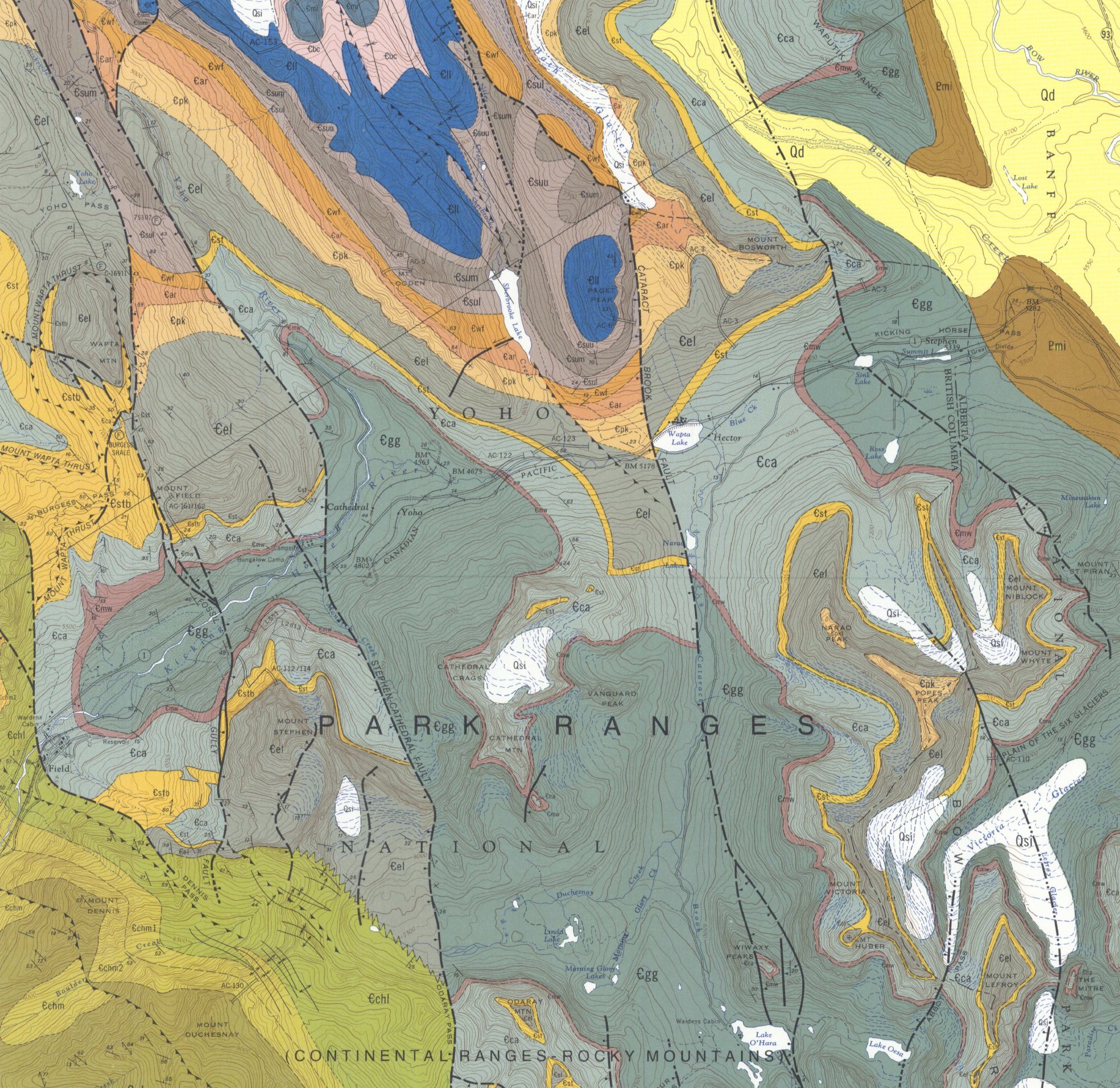
Look at Lake Louise, west half map by Price et al., 1980. The geologic map (opens in a new tab) and cross-sections (opens in a new tab) can be downloaded and printed on a poster to be able to better view geologic features. This area is very mountainous and has small valley glaciers.
Part 1: Map Information
- What are the contour intervals on this map? ___________________________________
- How would you identify a glacier versus a lake on this map? _______________________
- What is the scale of this map? ____________________________
Part 2: Cross-Sections
Find the two cross-section lines. Look at the northernmost cross-section between points labeled “6.”
- What is the highest point along this line? ________________________________
- What is the name of one prominent mountain along this cross-section? ___________________________________________________
- What is the elevation of the lowest point along this line? __________________________________________
- What is the total relief along the line of this cross-section? ____________________________________________________________
Part 3: Stratigraphic Column
- The Burgess Shale quarry locality is labeled with an F. It occurs north of the town of Field, to the west of Mount Field.
- What is the name of this formation? _______________________
- What is its color? __________________________
- What is its map symbol? __________________________
- What is its rock type? __________________________
- What is the general strike of this unit? __________________________
- What is the general dip of this unit? __________________________
- Look another unit either stratigraphically below or above the Burgess Shale location.
- What is the name of this formation? __________________________
- What is its color? __________________________
- What is its map symbol? __________________________
- What is its rock type? __________________________
- What is the general strike of this unit? __________________________
- What is the general dip of this unit? __________________________
- Which of these two formations is thicker? __________________________
- Which of these is made of resistant rocks? __________________________
Part 4: Structures and Correlation
- What type(s) of brittle structures are in the general vicinity of the Walcott quarry in the Burgess Shale unit? ___________________________________________________________________________
- What type of natural disaster do you think a gravity fault is associated with? ___________________________________________________________________________
- Using the schematic stratigraphic relationships, what formations are time correlative with the Burgess shale? ___________________________________________________________________________
- On the eastern edge of the map lies the oldest formation in this map area, the Proterozoic Windermere Group. You may remember a correlative unconformity, the Great Unconformity above the Vishnu Schist and Zoroaster Granite in the Grand Canyon (Figure 2.25) or a similar unconformity in Central Texas seen at Slaughter Gap. What type of unconformity occurs between the Windermere Group and the overlying lower Cambrian Gog Group? ___________________________________________________________________________
- Critical Thinking: Looking at this map, are there any areas you think might be good to find additional fossils equivalent to the Burgess shale fauna? When you propose an area, you need to consider several factors such as ease of access as even Walcott quarry is about 8 miles from a road and involves a steep climb. Also, avoid outcrops that may be close to faults. In addition, locations down low may be forested and not have any exposed rocks. ___________________________________________________________________________
Additional Information
Exercise Contributions
Virginia Sisson, Daniel Hauptvogel, Carlos Andrade, and Joshua Flores
References
Billingsley, G. H., 2000, Geologic Map of the Grand Canyon 30’ x 60’ Quadrangle, Coconino and Mohave counties, northwestern Arizona, U. S. Geological Survey, Geological Investigations I-2688 Map and Pamphlet. Public Domain
Price, R.A., Cook, D.G., Aitken, J.D., and Mountjoy, E.W., 1980, Geology, Lake Louise (west half), west of fifth meridian, British Columbia-Alberta. Geological Survey of Canada, “A” Series Map 1483A, 1980, 2 sheets, https://doi.org/10.4095/108873 (Open Access)
, , , and (2003), Tectonic shortening and topography in the central High Atlas (Morocco), Tectonics, 22, 1051, doi:10.1029/2002TC001460, 5.
Google Earth Locations
used to describe the orientation of a rock bed, fault, fracture, cuestas, igneous dikes, and sills.
the path of a fluid, most commonly a river or river delta
have a winding course, in geology used to describe rivers or streams
a remote sensing method that uses pulsed laser light to measure distances to the Earth
A geologic feature which is composed of layers with a convex form
A downward closing fold
a plane that divides a fold as symmetrically as possible. This may be vertical, horizontal, or inclined at any angle
a structural discontinuity in the Earth's crust or upper mantle. It forms as a response to inhomogeneous deformation partitioning strain into high-strain zones. Intervening blocks are relatively undeformed
rock that originated at a distance from its present position
rock formed in its present position
a remnant of a nappe after erosion has removed connecting portions of the nappe
this is used to emphasize vertical features, which might be too small to identify relative to the horizontal scale. Many geological cross-sections have no vertical exaggeration
a supercontinent that existed from the Neoproterozoic and began to break up during the Jurassic and ended in the Eocene
sedimentary rocks consisting of sandstone, siltstone, and shale, that are predominantly red in color due to the presence of ferric oxides. These can be deposited in both continental and marine paleoenvironments
a domed rock formation in which a core of rock has moved upward into overlying strata. These typically form when low-density material such as magma or salt flows upward
a glacier that begins at cirque at the head of a valley head or in a plateau ice cap and flowes downward between the walls of a valley. This erosion results in U-shaped valleys
