Chapter 3: Geologic Time

Daniel Hauptvogel; Virginia Sisson

Chapter 3: Geologic Time

The 2^nd edition is now available! Click here.

Learning Objectives

The goals of this chapter are to:

Illustrate the immense scale of geologic time
Summarize the geologic time scale
Explain the principles of relative dating and unconformities
Apply principles of relative and absolute dating to determine the ages of rocks

3.1 Introduction

Earth is 4.543 billion years old. That’s 4,543,000,000 years, an amount of time so immense that it’s challenging to grasp just how long it is. To put this into perspective, if the average human lifespan is 80 years, the Earth has been around for 57,000,000 lifetimes. Or if you have a penny for every year the Earth has been around, you would have $45.4 million! Constantly writing out millions and billions of years is time-consuming, so when geologists talk about ages, they use a few abbreviations. The symbols ka (thousands), Ma (millions), and Ga (billions) refer to points in time like a date. For example, the dinosaur extinction occurred at 66 Ma. Geologists also use other abbreviations for lengths of time, including ky, kya, kyr, and k.y. for thousands of years; my, mya, myr, and m.y. for millions of years; and by, bya, byr, and b.y. for billions of years. All four varieties of abbreviations mean the same thing in this case. Here, you would say the dinosaurs have been extinct for 66 myr. If this sounds confusing, you’re not alone because even some geologists use all of the abbreviations interchangeably. There is a debate amongst geologists, and other sciences, over the notation used for geologic time.

Fun fact: The Tyrannosaurus rex was one of the last dinosaurs to evolve about 70.6 Ma (a specific date). The first dinosaurs evolved about 230 Ma (a specific date), 159 myr (a length of time) before T-rex evolved. We are closer in time to the T-rex than the T-rex is to its earliest dinosaur ancestor! See the difference in abbreviations yet?

3.2 Geologic Time

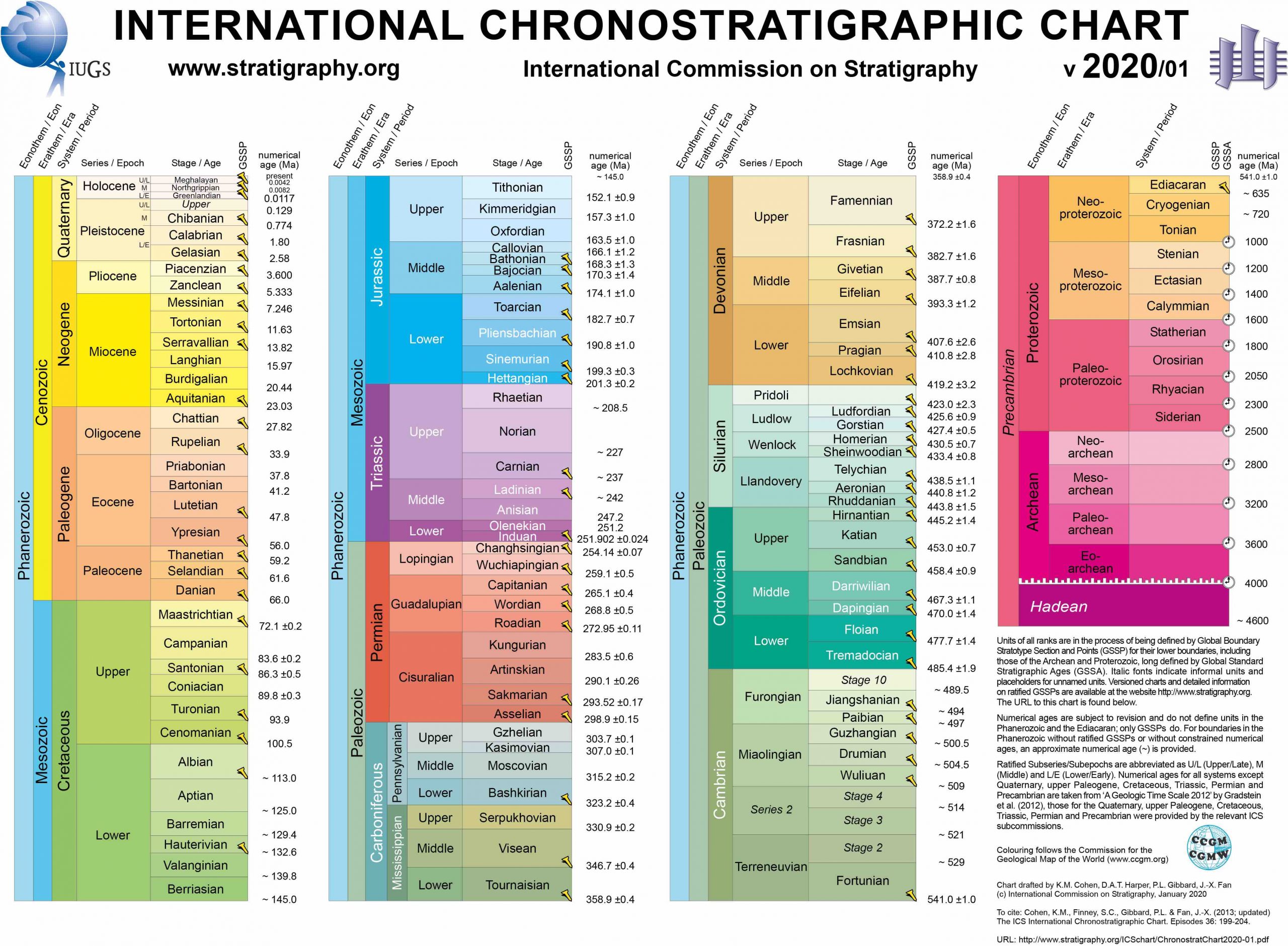
Since 4.54 byr is a large chunk of time, geologists have divided it into more manageable chunks by creating a time scale. The commonly accepted time scale comes from the International Commission on Stratigraphy (Figure 3.1). It is continually revised as new research fine-tunes numbers between time scale divisions. The one in Figure 3.1 is the most up-to-date at the time of this writing and will be referenced throughout this manual. The divisions on the time scale are often based on significant events that have taken place tectonically, biologically, or climatically, and the numerical ages are derived from radiometric dating of rocks, minerals, and fossils.

Geologic time is first divided into eons; these are the Hadean, Archean, Proterozoic, and Phanerozoic. The first three eons are often referred to as the Precambrian, which we’ll call a “super” eon. The eons are subdivided into eras, and eras are subdivided into periods, and periods into epochs, and epochs into ages. For the purposes of this lab manual, we will refer to this nomenclature. You’ll notice there is a second way to refer to these divisions on the time scale. The difference between the two is discussed here, but it is not important for our purposes. Throughout this lab manual, you will mainly see us referencing periods of geologic time.

The geologic timescale is broken up into different sections and subsections. — Figure 3.1 – The geologic time scale subdivided by eon, era, system, series, epoch, and stage. What do you observe about each period of time? It is simple; they are color-coded. We will use these standard colors throughout this lab manual. The golden spikes at age boundaries indicate a specific place used to define the age boundary. Image credit: International Commission on Stratigraphy.

Exercise 3.1 – Making Your Own Geologic Time Scale

Many depictions of the geologic time scale don’t show the divisions of geologic time on the same scale. Look at the time scale in Figure 3.1, for example. The far-right column goes from 4.6 Ga to 541 Ma; that’s about 4 billion years of history in one small column! The other three columns make up the remaining 500 myrs. The reason for this is that geologists know much more about the last 500 myrs of Earth’s history than the first 4 byrs. So, let’s make a geologic time scale where all geologic time is shown at the same scale.

Using a 2.5 m long roll of paper, create your own geologic time scale using the following scale: 1 cm = 20 million years. For the purpose of this exercise, round Earth’s age to 4.6 Ga and use a tick mark spacing of every 100 myrs.
Label the Precambrian and its associated eons.
Label the Phanerozoic eon and its associated eras and periods.
For the Cenozoic era, label the epochs.
Table 3.1 is a list of some major events in Earth’s history. On one side of your time scale, label when you think these events occurred using a color of your choice.
Using a cell phone or laptop, look up when these events actually occurred and label them on the other side of your time scale. Label physical events in one color and biological events in a different color. Some of the events will have a range of ages.

How close were your guesses?

Table 3.1 – A list of major events in Earth’s history
Formation of Earth’s Moon	Great oxidation event
Dinosaur extinction	Formation of the Himalayan Mountains
First fossil evidence of life	First homo sapiens
First fish	First mammals
First reptiles	First amphibians
First major glaciation, called Snowball Earth	End of the last ice age
Breakup of Pangea	Formation of Rocky Mountains
Earliest trace of life (bacteria)	Oldest oceanic crust

Come up with a mnemonic device to help you remember the periods of geologic time in the Phanerozoic Eon. For example, did you know that the word “scuba,” as in scuba divers, is actually a mnemonic device that stands for Self-Contained Underwater Breathing Apparatus?

Table 3.2 – Abbreviations for the Geologic Time Scale
Geologic Time Period	Abbreviation
Quaternary	Q
Neogene	Ng
Paleogene	Pg
Cretaceous	K
Jurassic	J
Triassic	T_R
Permian	P
Carboniferous	C
Devonian	D
Silurian	S
Ordovician	O
Cambrian	Ꞓ
Neoproterozoic	Z
Mesoproterozoic	Y
Paleoproterozoic	X
Archean	A

Geologists use abbreviations to refer to the different portions of geologic time (Table 3.2), particularly on geologic maps. A few of these abbreviations may seem puzzling because the abbreviation isn’t always the first letter of the name. Carboniferous got the “C”, so Cambrian got a C with a slash through it “Ꞓ“. This left Cretaceous with a “K.” Tertiary had originally received the “T”, which left Triassic to be symbolized with a T that had an R subscript. In 2003, “Tertiary” was stricken from the geologic timescale and replaced by the Paleogene and Neogene. You will still see “T” on older maps for Tertiary, and some geologists still use the term today. So, be careful! There were already some M’s and P’s; so, Proterozoic eras were assigned as X, Y, and Z.

Geologists use two methods for dating events in Earth’s history. The first is called relative dating, meaning how events relate to each other in time, or more plainly, they figure out the sequence of events (what came first, second, third, etc.). Relative dating has no regard for numerical ages. The second method is absolute dating, where geologists use radioactive isotopes to figure out the numerical age of a rock or mineral.

3.3 Relative Dating and Correlation

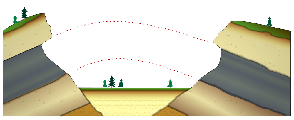
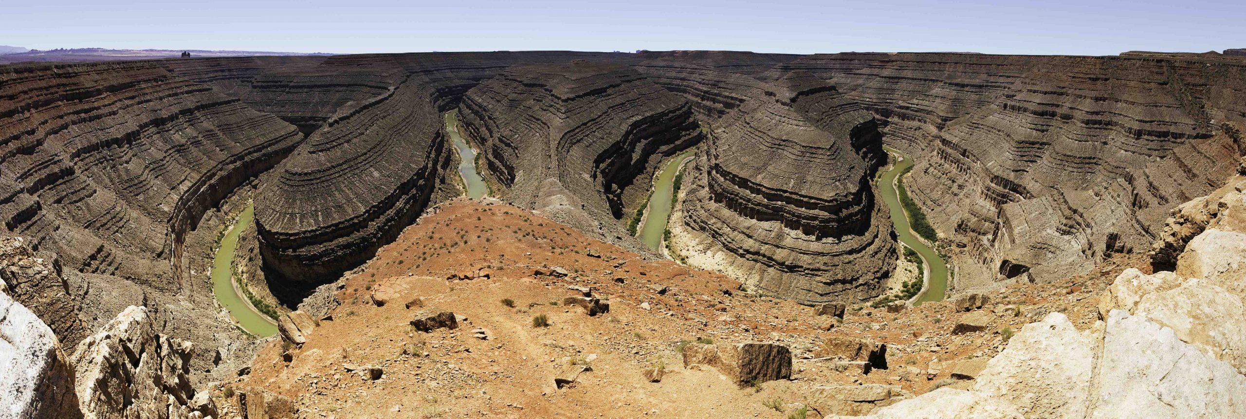
There are several principles geologists use for relative dating. The first four principles were developed in the 17th century by an early geologist named Nicolas Steno, three of which pertain to sedimentary rocks. The first is the law of superposition, which states that in layers of horizontal sedimentary rocks, the oldest rock layer is at the bottom, and the youngest is at the top (Figure 3.2). The second rule is the principle of original horizontality, which says that layers of sediment are originally deposited horizontally (Figure 3.2). So, any tilting or folding of the rock occurred after it was deposited (Figure 3.3). The third principle states that layers of sedimentary rock are continuous, and anything that interrupts the layer (like a river or canyon) happened after the rock formed. This is called the principle of lateral continuity (Figures 3.4 and 3.5).

Outcrop of sedimentary rocks that shows the principles of superposition and original horizontality. — Figure 3.2 – Horizontal layers of red sedimentary rocks from the Moenkopi and Chinle Formations from the Triassic period in the Virgin River Valley near Zion National Park. Layers of sedimentary rock are originally deposited horizontally, with the oldest layer at the bottom. This shows both the principles of superposition and original horizontality. Image credit: James St. John, CC-BY.

Layers of sedimentary rock titled at an angle. The tilting occurred after the layers were deposited horizontally. — Figure 3.3 – These are tilted layers of the Moenkopi Formation from the Lower Triassic, just south of Split Mountain, Dinosaur National Monument in Utah. They were originally deposited horizontally and were titled at some point in geologic time. Image credit: James St. John, CC BY.

Depiction the principle of lateral continuity across a valley. — Figure 3.4 – A depiction of the principle of lateral continuity. The layers of rock on one side of this valley were once connected to the same rocks on the other side. The valley was carved after these rocks were deposited. The dashed red lines show how the units were connected. Image credit: Wikimedia user Wouldloper, Public Domain.

Panoramic view of the San Juan River that shows lateral continuity as layers of rock would have connected across each canyon. — Figure 3.5 – A panoramic view of meanders in the San Juan River cutting through layers of sedimentary rock in Goosenecks State Park, southwestern Utah. If you look carefully, you can trace layers of sedimentary rock that have been cut by the river across the entire image; an example of lateral continuity. Image Credit: Gernot Keller, CC BY.

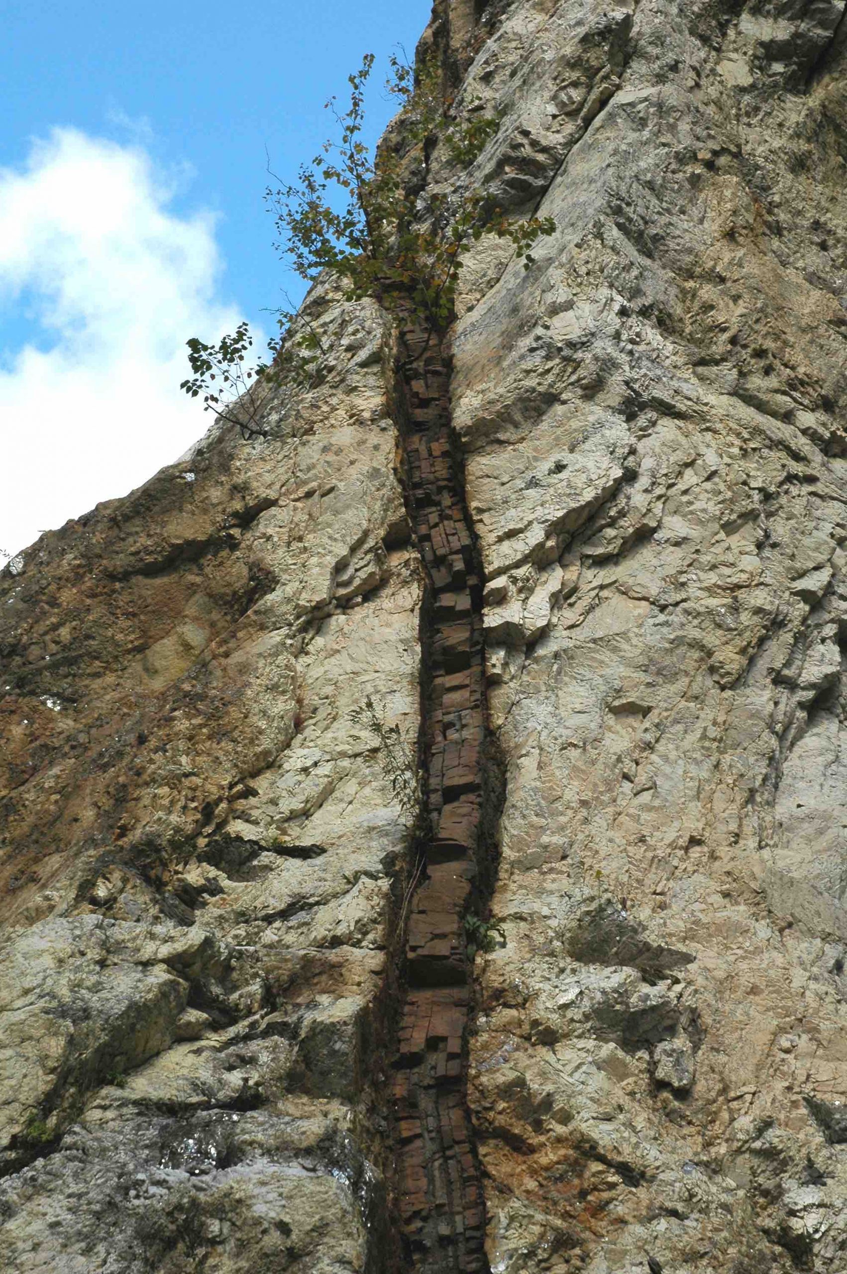
Steno’s fourth principle is cross-cutting relationships. This principle is used when other geologic events cut through sedimentary rocks, like an igneous dike or a fault. This principle basically states that when a geologic event cuts across another, the event doing the cutting is younger than the one being cut (Figure 3.6). For example, if sedimentary rocks are cut by an igneous dike, the igneous dike is younger than the sedimentary rocks it’s cutting through. The same can be said of a fault that cuts through any rock; the fault has to be younger because the rocks had to exist first to be faulted.

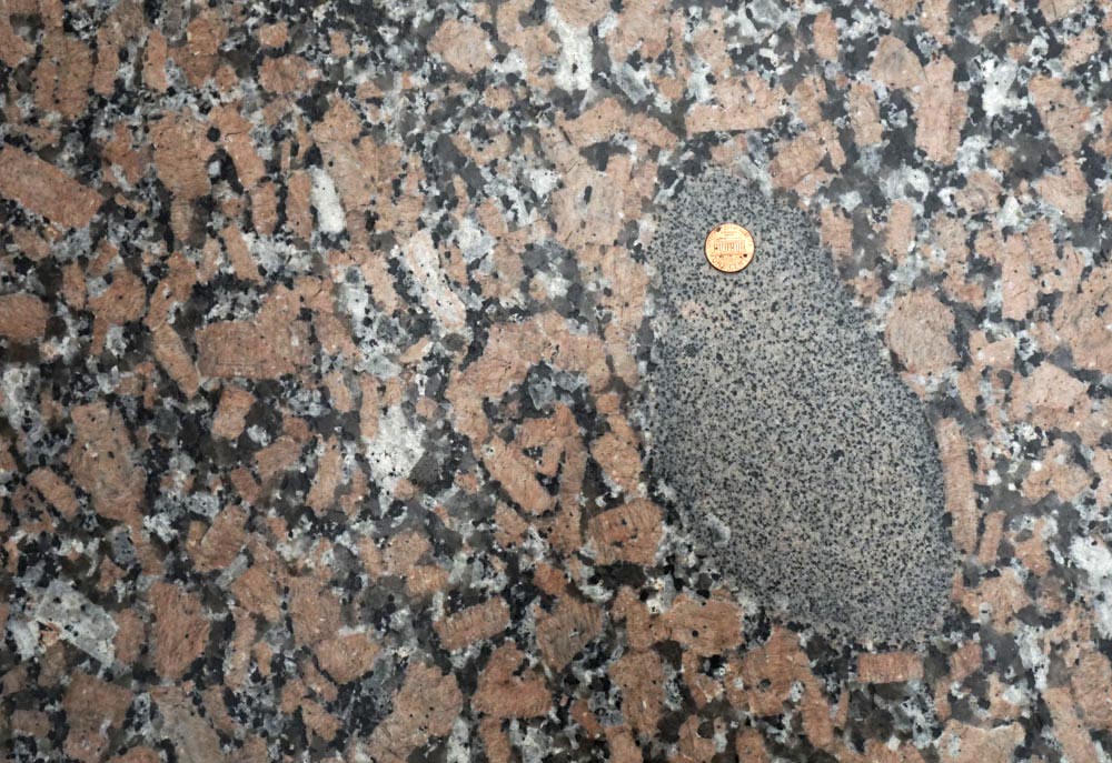
A mafic dike cutting through granitic pegmatite in Ruggle's Mine, New Hampshire. — Figure 3.6 – A mafic dike (dark rock) cutting through granitic pegmatite (light rock) in Ruggles Mine, New Hampshire. To determine which is younger, look to see which unit cross-cuts the other. Since the mafic dike is cutting through the pegmatite, the dike is younger by the principle of cross-cutting relationships. Image credit: James St. John, CC BY.

Some 200 years later, the fifth principle of relative dating was developed by Charles Lyell called the principle of inclusions. This principle explained that a clast, or a different-looking rock that is contained inside of another rock, is older than the rock that contains it (Figure 3.7). How can this happen? Originally, a mafic magma was cooling quickly, producing the finer-grained mafic rock in the middle of Figure 3.7. Then, something happened to change the chemistry of the magma to felsic and slowed the cooling rate to produce the surrounding, coarse-grained granite. The mafic rock formed first, and then the felsic rock formed around it.

This image shows the principle of inclusions. The dark colored inclusion is older than the surrounding granite. — Figure 3.7 – A mafic inclusion in granitic rock. Inclusions are older than the surrounding rocks. A penny shows the scale of the image. Image credit: Marli Miller, CC BY.

Unconformities

Simply speaking, an unconformity is a pattern that you look for in a group of rocks that tells you erosion has taken place. Rocks exposed on the Earth’s surface are affected by physical and chemical weathering processes that work to break them into smaller pieces or dissolve them in water. This material is then transported away by wind, water, or ice, a process known as erosion. Many people use weathering and erosion interchangeably, but they do mean different things: weathering is the breakdown of rocks, while erosion removes the broken down material.

There are four types of unconformities, and each forms in a slightly different way (Figure 3.8). They all involve sedimentary rocks, changes in sea level, and/or uplift from an orogeny. Each unconformity tells a unique story of the geologic history of the area they’ve been found.

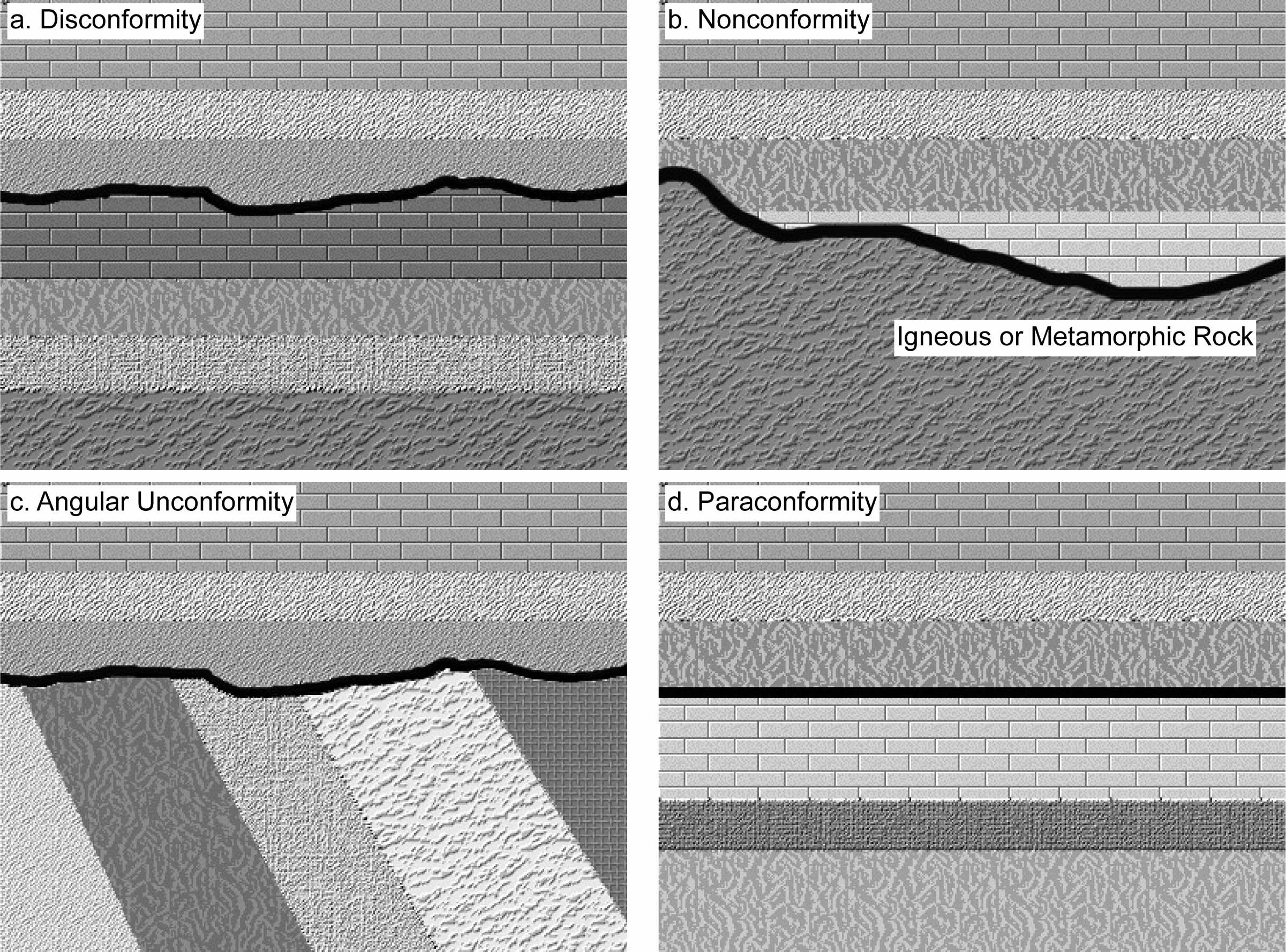
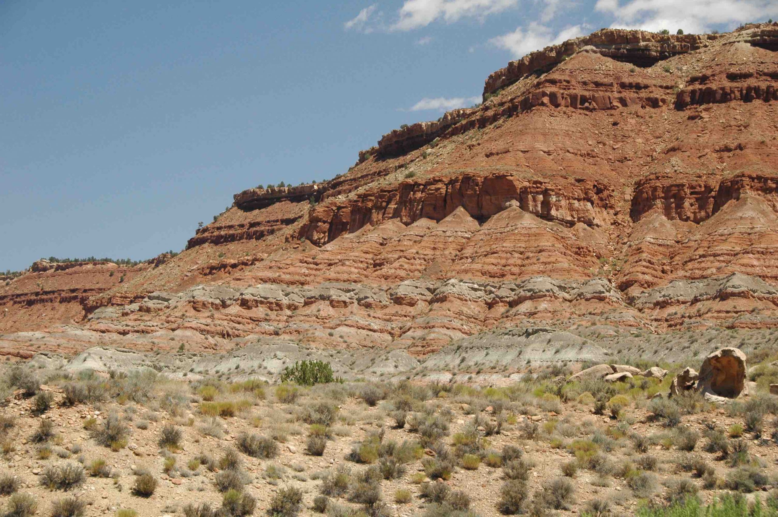
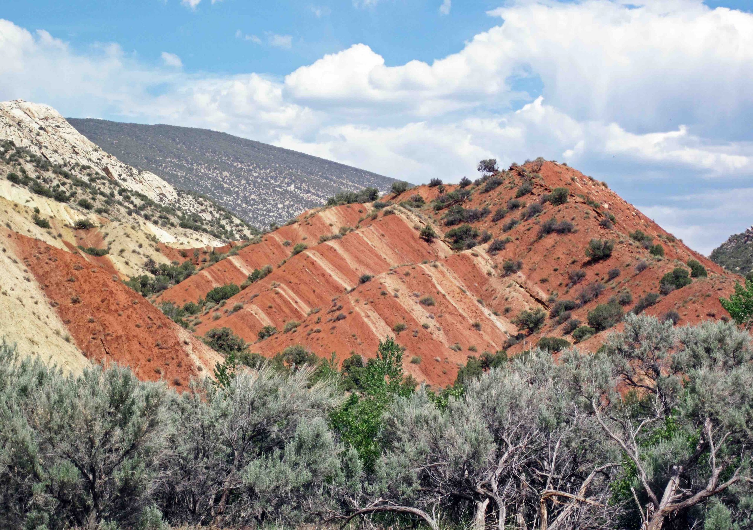
Four images showing different types of geological unconformities. — Figure 3.8 – Types of unconformities. (a) Disconformity; (b) Nonconformity; (c) Angular unconformity; (d) Paraconformity. Image credit: Wikimedia user דקי, CC BY-SA.

A disconformity (Figure 3.8a) is an erosional surface where the rocks below the unconformity are much older than the rocks above. This type of unconformity typically forms when horizontal layers of sedimentary rock are deposited in a shallow marine environment; then sea level lowers to expose these rocks and allows erosion to occur; then sea level rises again, and new horizontal layers of sedimentary rock are deposited. Erosion removed some of the original rock, creating a large age gap between the rocks above and below the erosional surface. This age gap is the disconformity and is located at the contact point between the older rock and younger rock. Oftentimes the erosion process leaves behind evidence of river channels or soil development, which provide clues to geologists to locate the unconformity in what looks like a continuous succession of sedimentary layers.

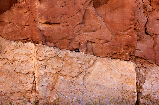
A nonconformity (Figure 3.8b) forms when igneous or metamorphic bedrock is eroded, and then horizontal layers of sedimentary rock are deposited directly on top of it. The unconformity is where the bedrock meets the sedimentary rock. For example, when a mountain belt is eroded below sea level, and afterward sediments are deposited on top of the igneous or metamorphic rock, the contact is a nonconformity.

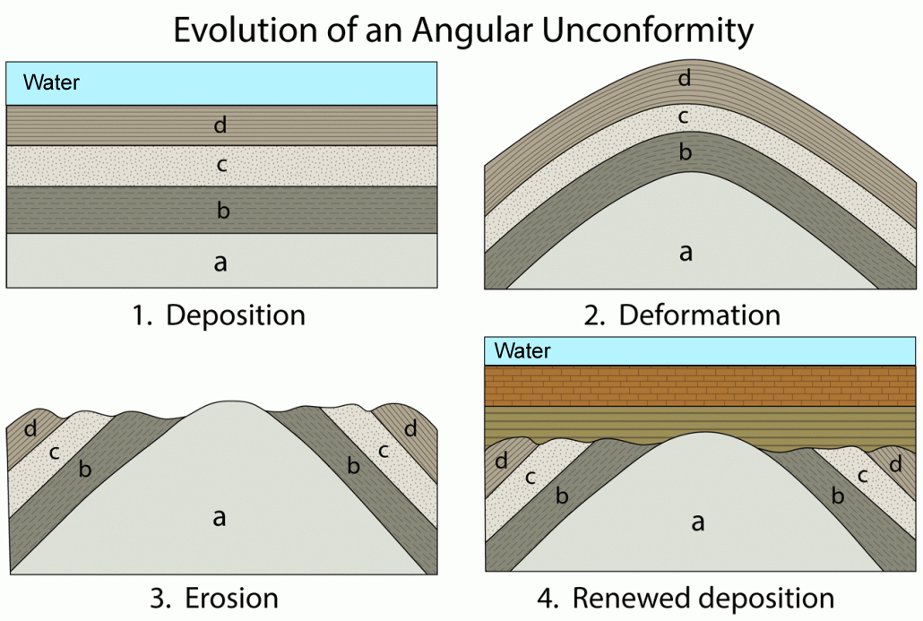
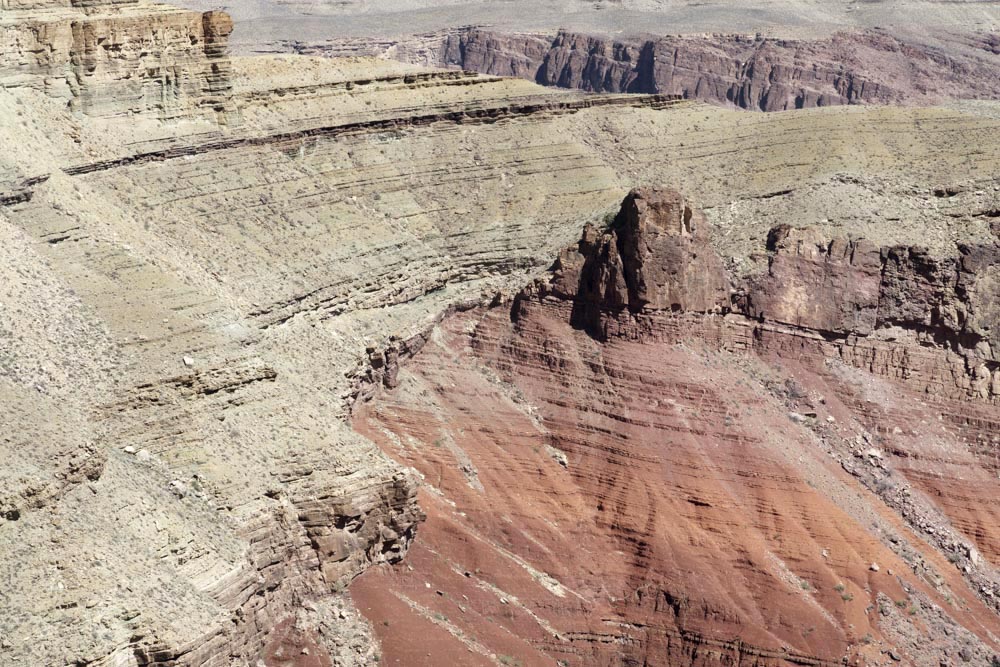
An angular unconformity (Figure 3.8c) is created when horizontal layers of sedimentary rock lie on top of tilted layers of sedimentary rock. The most famous angular unconformity is from Siccar Point in Scotland. Figure 3.9 shows the process of creating an angular unconformity. For this to occur, sedimentary rocks deposited in the marine environment are lifted above sea level by an orogeny or similar event. The orogeny causes the sedimentary rocks to become tilted or folded. Since these rocks are exposed above sea level, erosion takes place. The rocks can either be eroded below sea level, or sea level can rise, which would allow new, horizontal layers of sedimentary rock to be deposited on top of the titled ones. This creates an angle between the younger, horizontal layers on top and the older, tilted layers below.

The four steps in this figure show the processes by which an angular unconformity forms. — Figure 3.9 – A depiction of how an angular unconformity forms. 1) Deposition of sedimentary rocks; 2) uplift and folding of the sedimentary layers; 3) erosion; 4) resumed deposition on top of the folded layers. Image credit: Utah Geological Survey, Public Domain.

A paraconformity (Figure 3.8d) is very similar to a disconformity, except the evidence for erosion is not present. Either no evidence of the erosion was left behind, or erosion didn’t happen, and instead, there was only a pause in sediment deposition. We know these occur because sediment above and below the paraconformity have been radiometrically dated and reveal a large gap in time.

Exercise 3.2 – Identifying Unconformities

The images in Table 3.3 are different types of unconformities (Figures 3.10-3.12). In the blank spaces provided next to the images, create a sketch for each unconformity, label where you think the unconformity is located, and identify the type of unconformity.

Table 3.3 – Worksheet for Exercise 3.2
Unconformity Image	Your Sketch
Figure 3.10 – Unconformity #1. Image credit: Marli Miller, CC BY.
Figure 3.11 – Unconformity #2. Image credit: Callan Bentley, used with permission.
Figure 3.12 – Unconformity #3. Image credit: Marli Miller, CC BY.

Exercise 3.3 – Practicing Relative Dating Principles

Part I

Now put all of the principles you’ve learned to work. Below are relative dating outcrop diagrams that represent sections of rock. Each letter represents the deposition of a different layer of sedimentary rock or geologic event.

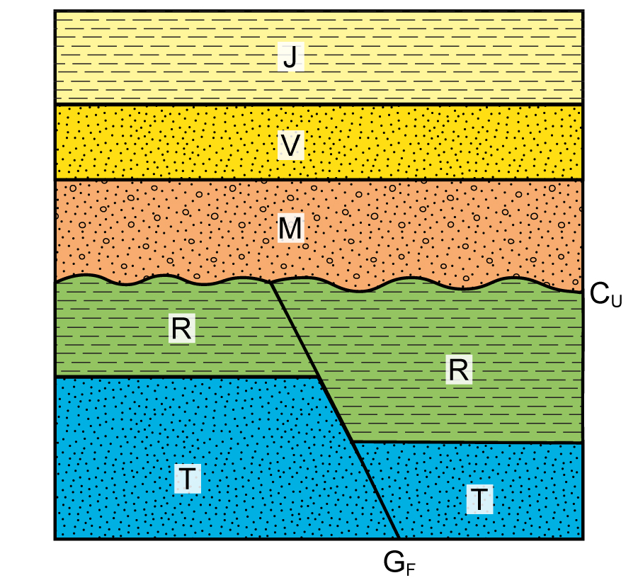
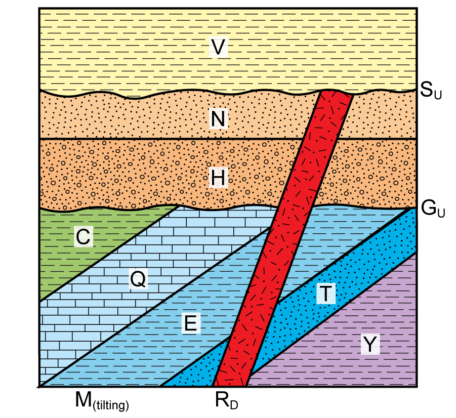
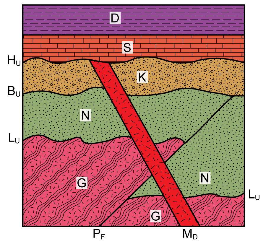
Use the principles of relative dating and unconformities to determine the sequence of events for each diagram in Table 3.4 (Figures 3.13-3.16).
Identify the type of each unconformity.

The symbols used to represent common types of rocks are standard USGS symbols. You will only see conglomerate, limestone, sandstone, shale, granite, and gneiss in this exercise. The subscript letters stand for igneous dikes (D), faults (F), and unconformities (U). The colors for each unit are from the geologic time scale shown in Figure 3.1. Hint: it is easier to start with the oldest event and work your way forward through time.

Table 3.4 – Worksheet for Exercise 3.3
Figure 3.13 – Diagram #1. Image credit: Daniel Hauptvogel, CC BY-NC-SA.	youngest oldest
Figure 3.14 – Diagram #2. Image credit: Daniel Hauptvogel, CC BY-NC-SA.	youngest oldest
Figure 3.15 – Diagram #3. Image credit: Daniel Hauptvogel, CC BY-NC-SA.	youngest oldest
Figure 3.16 – Diagram #4. Image Credit: Daniel Hauptvogel, CC BY-NC-SA.	youngest oldest

Part II

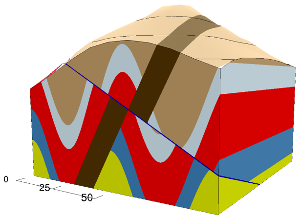
The web program Visible Geology lets you create block models with a complicated geologic history. An example of a diagram made with this website is in Figure 3.17. Answer the following questions using Figure 3.17:

Place the following in order from youngest to oldest: Fault, Dike, Folding. ______________________________
If the dike is 100 Ma, what is the age of the normal fault? ____________________

Figure 3.17 – Block diagram created using the website Visible Geology. Sedimentary strata are shown in yellow, blue, red, white, and tan. The dark brown is an igneous dike. The blue line is a fault. The dashed lines represent contour lines.

Part III

Create your own block model using the web program Visible Geology.

Your model should include 2 to 6 sedimentary layers. You may want to vary their thickness. Each rock type is assigned a unique color. You can also include an unconformity (angular, disconformity, or nonconformity).
You can include tilting, folds, thrusts, strike-slip faults, and normal faults.
You may want to include some igneous rocks as sills or dikes. If you include a dike or sill, you may want to assign it a specific age, such as 100 Ma. This numerical age can be used to give specific dates to events in this geologic history.
Include erosion at some point in your model.

When you are done with this, rotate the cube and decide which side has the easiest and most difficult history to assess. Or perhaps you made a model that is easy on all sides? Explain why there is this difference.
Create a geologic cross-section through your model from corner to corner. Draw a sketch of one of these cross-sections.

Cross-Section Sketch #1:
Sometimes geologists only have cliff faces or road cuts to investigate. Do you think you will get the same geologic history with this cross-section as one of the sides?
Now draw a quick sketch of one of the sides. Show it to one of your classmates and see if they can interpret its geologic history. If you included an igneous feature, assign it an age. If your colleague can’t get the history, give them some clues to help.

Cross-Section Sketch #2:

Exercise 3.4 – Using Relative Dating Principles

One of the ways geologists investigate Earth’s history is by imaging what is below Earth’s surface; this is called a seismic survey. It is done by sending sound waves into the ground or ocean. As these sound waves move through different layers of rock or sediment, some of the waves are reflected back toward the surface and recorded by geophones. Different types of sediments or rocks change the characteristics of the wave, such as its velocity. Geologists set up geophones that record these reflected waves and provide an “image” of what the subsurface looks like. The signals recorded are called the seismic amplitudes, a measure of the difference in rock properties between two layers. Seismic data is commonly converted to impedance, or hardness (this is not the same as Mohs hardness). The relative hardness can be positive, negative, or the same. Thus, many seismic sections will use three colors to better distinguish different strata.

Part I

The continental slope off of the north island of New Zealand is called the Hikurangi margin. Geoscientists wanted to explore this area to better understand the plate boundary by drilling a sediment core. The International Ocean Discovery Program (IODP) proposed to put a drill core at Site U1519, but first, they conducted a seismic survey (Figure 3.18) to assess the possibility of active thrust faults in the area.

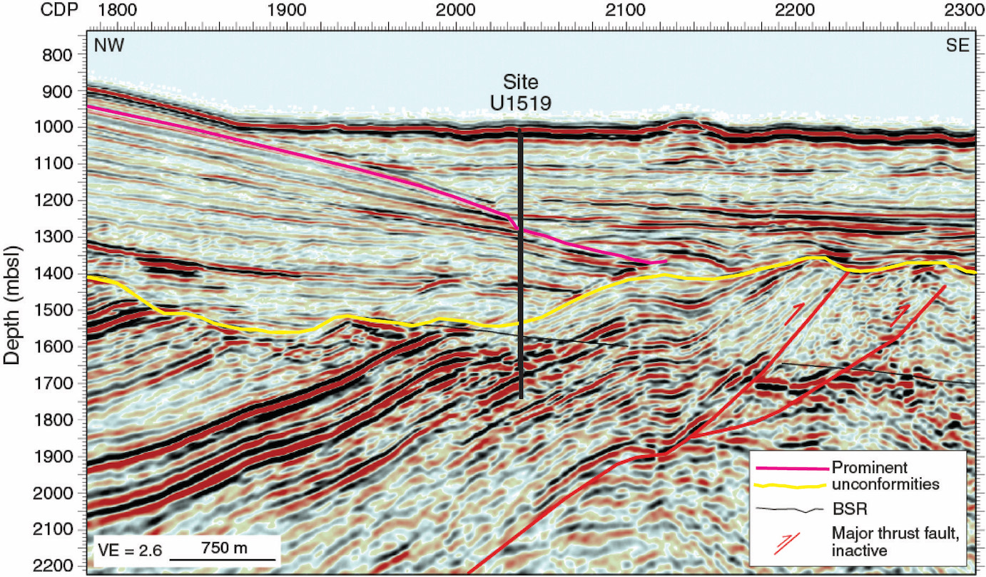
Figure 3.18 – Seismic profile for IODP Site U1519. There are two unconformities shown with yellow and pink lines. Also shown in a thin black line is the bottom simulating reflector (BSR). The black color is used for positive amplitudes, red for negative amplitudes, and white for zero amplitude. Image credit: Wallace et al., 2019 and IODP, CC BY.

What type of unconformity is the yellow line? ____________________
What type of unconformity is the pink line? ____________________
Critical Thinking: Do you think it would be safe to drill here? Explain your answer.

Part II

As the Pacific plate traveled over numerous hot spots, the basement of the Gulf of Alaska became riddled with seamounts. The seamounts have a variety of ages and sizes, as you can see in Figure 3.19. These are partially covered by a thick blanket of sediments up to 1.5 km thick.

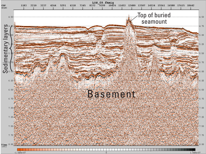
Figure 3.19 – Seismic profile from the Gulf of Alaska. Since this is a preliminary seismic section, it has not been processed to show depth. Instead, it shows two-way travel time in seconds for the seismic energy. The red, black, and white lines indicate sedimentary layers, whereas the red, black, and white dots represent the oceanic crust (basement). The sedimentary layers are more than 1.5 km thick. The same color scheme is used for seismic rock properties as in Figure 3.18. Image credit: USGS, Public Domain.

Identify two areas where faulting has taken place by outlining them in Figure 3.19.
Why is the contact between the crystalline basement and the sedimentary layers above it not considered unconformity?

Sedimentary Rock Correlation

The principles of relative dating allow geologists to compare seemingly similar groups of rocks separated by some distance. On a small scale, it’s as simple as saying that rocks on either side of a canyon are, in fact, the same and were once connected before the canyon formed, as in Figure 3.5. On a larger scale of kilometers to hundreds of kilometers, it can be comparing sets of sedimentary rocks that have similar patterns.

Exercise 3.5 – Correlating Layers of Sedimentary Rock

Geologists can correlate sedimentary rock units over great distances by matching patterns in the outcrops, called lithostratigraphic correlation. Figure 3.20 below contains two outcrop drawings of sedimentary rock outcrops that are separated by 100 km.

Draw lines that correlate the rock units across these two areas. You can color the units to help you.
One of these areas contains an unconformity. Mark the location of the unconformity in Figure 3.20.
What type of unconformity is it? _________________________
Critical Thinking: Are any other sedimentary layers missing from one of the outcrops? If so, explain why.

Two stratigraphic columns to be used for exercise 3.5. — Figure 3.20 – Two stratigraphic columns to be used in Exercise 3.5.

Fossil Correlation

Fossils present in sedimentary rocks can also be used for correlation. This usually involves a fossil assemblage, which is just the group of fossils found in a rock layer. By comparing fossil assemblages from one rock outcrop to another, geologists can determine how the outcrops relate to each other in age. This can tell geologists that layers of rock may have been deposited simultaneously or can be used to identify unconformities.

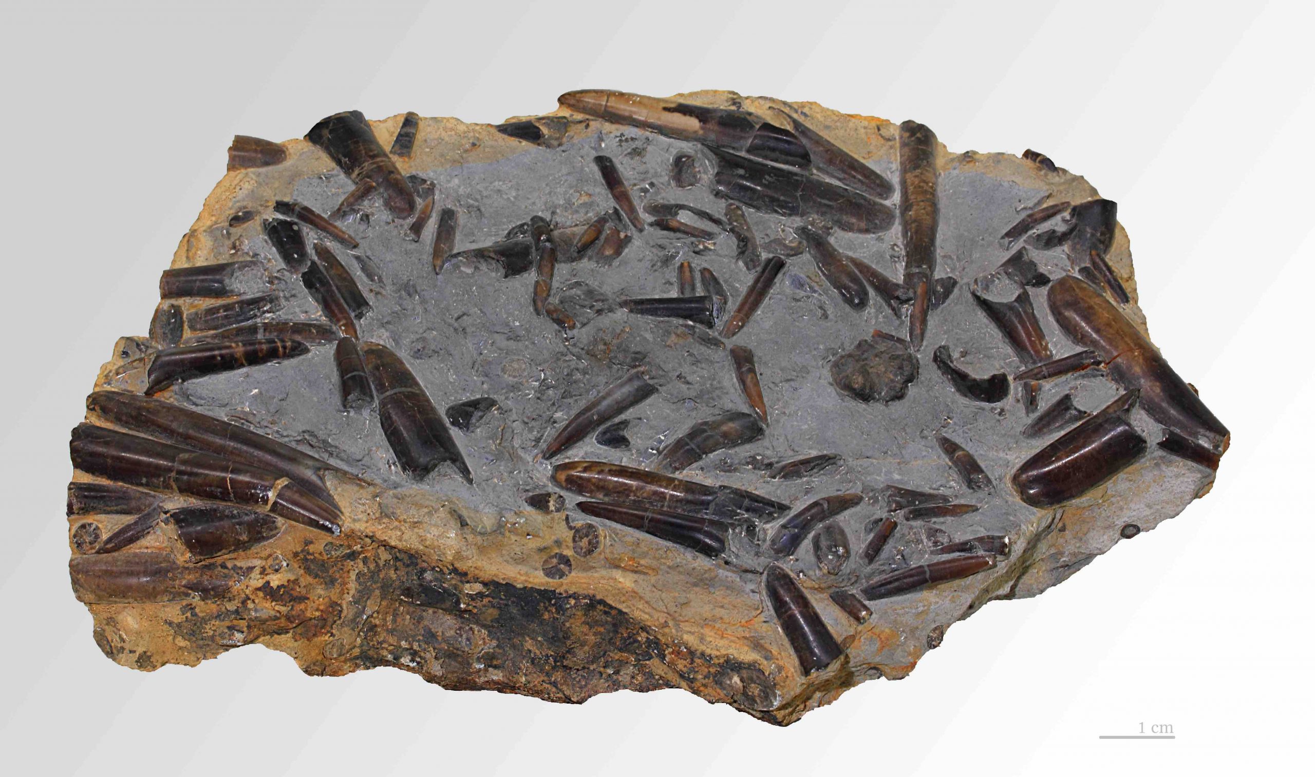
The belemnite fossils are the cone-shaped objects in this sedimentary rock. — Figure 3.21 – A sedimentary rock containing multiple belemnite fossils. These cone-shaped shells come from an extinct marine animal similar to a modern squid. Image credit: Wikimedia user PierreSelim, CC BY-SA.

Certain fossils, called index fossils, can be indicative of a narrow span of geologic time. These fossils are easily recognizable, abundant, existed for a short period of time, and had a wide geographic distribution. When you see an index fossil in a rock, it immediately gives you an idea of how old the rock is. For example, Belemnites (Figure 3.21), a type of cephalopod (squid), only existed during the Mesozoic era. So if you were to see a belemnite fossil in a rock, you know that rock is from the Mesozoic (between 252 and 66 Ma). We’ll have lots more on fossils in later chapters.

Exercise 3.6 – Using Fossils to Correlate Rocks and Interpret Age

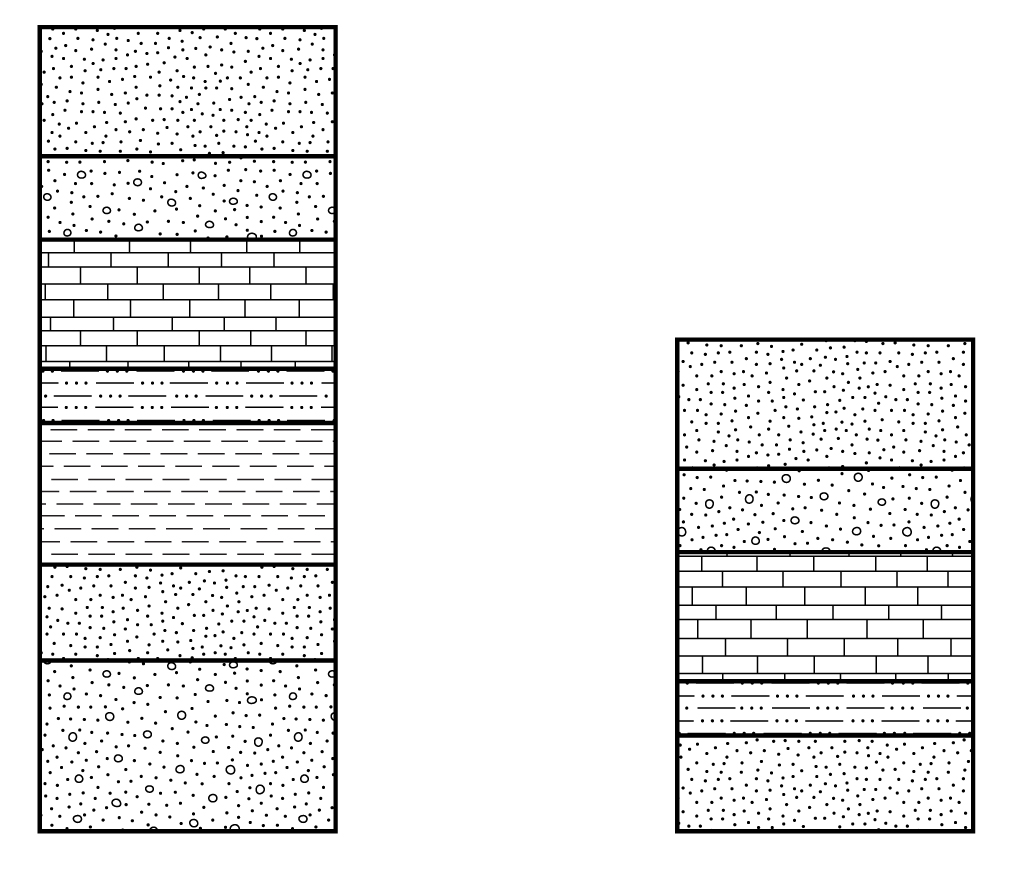
Fossils are very useful for geologic dating and correlation because the type of sediment deposited at a specific time in a region can vary. Sand particles (sandstone) can be deposited in one area, while clay particles (shale) can be deposited in another at the same time. This means that two different sedimentary rocks will have the same age. In this case, correlating the rock units is more difficult because geologists can’t tell they are the same age. This is where fossils can help because they can confirm the sedimentary rocks were deposited at the same time, called biostratigraphic correlation. If both rock layers were deposited at the same time, then they should contain the same fossils.

Correlate the sedimentary layers in Figure 3.22 based on the fossils they contain.
Label where any unconformities could be interpreted.

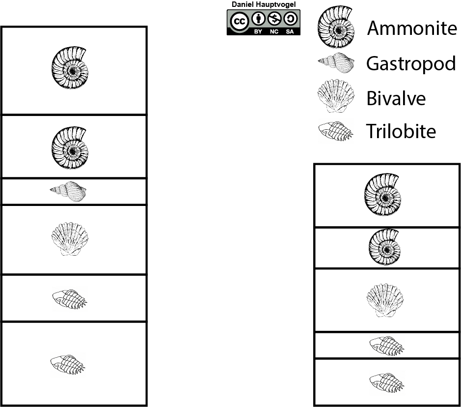
Figure 3.22 – Two stratigraphic columns for Exercise 3.6.
You can also use the assemblage of fossils in rocks to correlate sedimentary layers and determine age. Correlate the rock layers in Figure 3.23 based on the groups of fossils that are found.
Label where any unconformities could be interpreted.

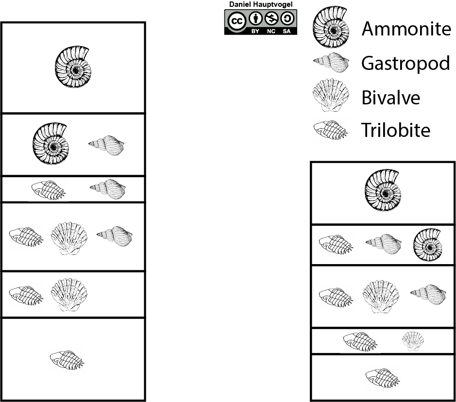
Figure 3.23 – Image for Exercise 3.6.
Suppose the fossils have age ranges as shown in Figure 3.24. Label the geologic periods for each layer of sedimentary rock in both columns of Figure 3.23.

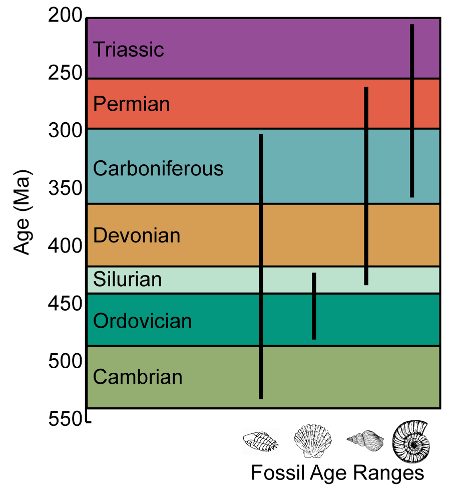
Figure 3.24 – Geologic time scale from Cambrian to Triassic that shows fossil age ranges for Exercise 3.6. The age span for each type of fossil is shown as a black bar above the sketch of the fossil.
Which of the fossils is the least useful for dating? __________________________
Which of the fossils is the most useful for dating? __________________________

*Note the fossil age ranges in this exercise are fictional and used for educational purposes only.

3.4 Radiometric Dating

Geologists can determine numerical ages for the formation of rocks, minerals, and some fossils using radioactive isotope systems. Does radioactivity sound scary? It can be, but what we’re talking about is happening on such a small scale that you don’t have to worry. The next few paragraphs are a bit technical, but we will try to break it down for you.

An isotope is an atom of an element with a different number of neutrons than protons in its nucleus. For example, a typical carbon atom on the periodic table of elements should have six protons and six neutrons in its nucleus, called carbon-12. Some atoms of carbon can have an extra neutron in the nucleus, called carbon-13, and some can have two extra neutrons in the nucleus, called carbon-14. If an atom has too many neutrons in its nucleus, it can become unstable because the nucleus has too much energy; this is called a radioactive isotope. Carbon-14 is a radioactive isotope. Just as the periodic table of elements summarizes the most important information of every element, there are periodic tables of isotopes that include all the possible isotopes for each element and their relative abundance and properties.

Radioactive isotopes decay to more stable atoms by way of alpha, beta, and/or gamma decay. We don’t need the particulars of these decay processes, but in short, radioactive atoms can gain or lose protons, neutrons, and electrons or release energy in other forms to become stable. Carbon-14 radioactively decays to nitrogen-14, a stable product. This ThoughtCo article gives a very simple explanation of why atoms become radioactive if you want more information.

Table 3.5 – Common isotope systems used for radiometric dating and their half-lives
Parent Isotope	Stable Daughter Product	Half-life
Uranium-238	Lead-206	4.5 billion years
Uranium-235	Lead-207	704 million years
Thorium-232	Lead-208	14.0 billion years
Rubidium-87	Strontium-86	48.8 billion years
Potassium-40	Argon-40	1.25 billion years
Samarium-147	Neodymium-143	106 billion years
Carbon-14	Nitrogen-14	5,730 years

Radioactive isotopes don’t immediately decay to a stable form because it’s a spontaneous process, so it’s impossible to predict when and which atom will decay. It’s like corn kernels popping in a popcorn maker, you don’t know when a kernel will pop, but you know it will happen. Scientists have measured the average rate at which radioactive isotopes decay and describe this rate with the term half-life. Half-life is the time it takes for half of the unstable atoms (parents) to decay to stable forms (daughters). The length of time for a half-life is different for each isotope system. For example, the half-life for carbon-14 is 5,730 years, but the half-life for potassium-40 is 1.25 byrs. In a sample with 1 million atoms of carbon-14, 500,000 of these atoms are expected to decay over the course of 5,730 years. Table 3.5 contains common isotope systems and their half-lives.

Using radioactive isotope systems, geologists can determine quantitative, numerical ages for geological materials and such as rocks, minerals, and fossils. To calculate the age of a geologic material, geologists analyze the material’s chemistry and figure out the ratio between parent and daughter atoms. The ratio tells geologists how many half-lives, or what fraction of a half-life, has passed. If you know the ratio between parent and daughter atoms and the rate of decay for that isotope system, you can calculate how old geologic material is.

Geologists use a few assumptions with radiometric dating. One assumption is that when the rock or mineral first formed, there were no daughter atoms present. This means all of the daughter atoms found in the rock had to come from radioactive decay. The second assumption is that the rock or mineral was a closed system. A closed system means there was no addition or removal of elements at any point because that could alter the parent-daughter ratio and therefore affect the age you calculate. With that being said, geologists know that these assumptions may be incorrect for some of the material they work with, and they have methods that can help correct these issues. But that is beyond our scope. That’s it for the technical stuff.

Radiometric dating tells you different things depending on which geologic material you’re studying. For minerals in igneous rocks, the radiometric age tells you when the mineral crystallized from magma. In metamorphic rocks, the radiometric age of some minerals can give you the age metamorphism took place, but some isotope systems are not affected by metamorphism and can still tell you the age the minerals originally crystallized in the protolith. So, you can determine when the protolith formed and when it became metamorphosed. For minerals in sedimentary rocks, the radiometric age only tells you when that mineral crystallized or metamorphosed in its original rock; it doesn’t tell you when the sedimentary rock formed. The only way to determine the age of sedimentary rocks is to combine the principles of relative dating with radiometric dating of igneous or metamorphic events that cross-cut the sedimentary rocks, such as a dike. Ages of sedimentary rocks can also be determined from fossils. Note: It is possible to radiometrically some sedimentary rocks younger than one million years old, but there are no useful isotopes that can be used on older sedimentary rocks.

Exercise 3.7 – Calculating Radiometric Ages

To determine the age of a mineral or rock, geologists need to know a few things. First, they need to know how long a half-life is for the isotope system being used. Second, they need to know the ratio of parent to daughter isotopes in the mineral, which is measured using scientific instruments like a mass spectrometer.

The standard radiometric age equation is: t=ln(1+(D/P))÷λ

t = time (age of the material)
ln = natural log (a function on your calculator)
P = parent ratio (this is measured)
D = daughter ratio (this is measured)
λ = lambda is the decay constant (different for each isotope system, a function of the half-life)

Let’s get some practice by calculating the ages below:

Complete the following calculations to determine the ages of minerals in Table 3.6 (Hint: most cell phones have additional calculator functions when you turn it horizontal. There are also free scientific calculator apps in the Apple and Google stores.)

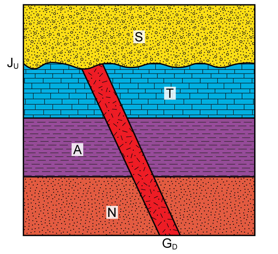
Table 3.6 – Worksheet for Exercise 3.7
Isotope System	Decay Constant	Parent : Daughter Ratio
Carbon-14	1.21×10^-4	1 : 1.3
Potassium-40	5.34×10^-10	1 : 0.25
Uranium-235	9.72×10^-10	1 : 2.34

Look back to Figure 3.16. Let’s say a geologist collected a sample of G (gneiss) and M_D (dike) to radiometrically date, with the ultimate goal of trying to constrain ages in this region. She used the potassium-40 isotope system to date metamorphism of hornblende grains and measured a parent-daughter ratio of 1:0.89. She used the uranium-235 isotope system on zircon grains for the igneous dike and measured a parent-daughter ratio of 1:0.28.
1. How old is the gneiss? ____________________
2. How old is the igneous dike? ____________________
3. What is age range of the fault P_F? ____________________
4. What is the age range of sedimentary layers S and D? ____________________

3.5 Other Uses for Geologic Dating

Dating in geology has many uses besides determining when a rock or mineral formed. One common use for dating is determining the source rock for sediment, which is called provenance. Interpreting sediment provenance can tell a geologist a lot about the history of an area, including where the sediment came from, where erosion was taking place, and how sediment was transported. Dating of certain sediment grains can also tell geologists when rocks were uplifting during an orogeny. Geologic dating principles can even be used on other planets.

Exercise 3.8 – Using Geologic Dating to Interpret Sediment Provenance

Even though radiometric dating on mineral grains in sedimentary rocks doesn’t give you the age the sedimentary rock formed, it still tells you very useful information about the area’s geologic history. One such use is determining the sediment provenance, which is the source rock of the sediment. Remember that the age you determine from sediment grains is the age they formed in their original source rock.

Let’s say you collect some biotite grains from the bottom of the lake in Figure 3.25, and you want to figure out where they came from. There are two potential sources for those grains: a set of metamorphic rocks to the west and a set of granites to the south. Little is known about the geology in this area, so you need to figure out the ages of the potential source rocks and determine where the lake sediment came from.

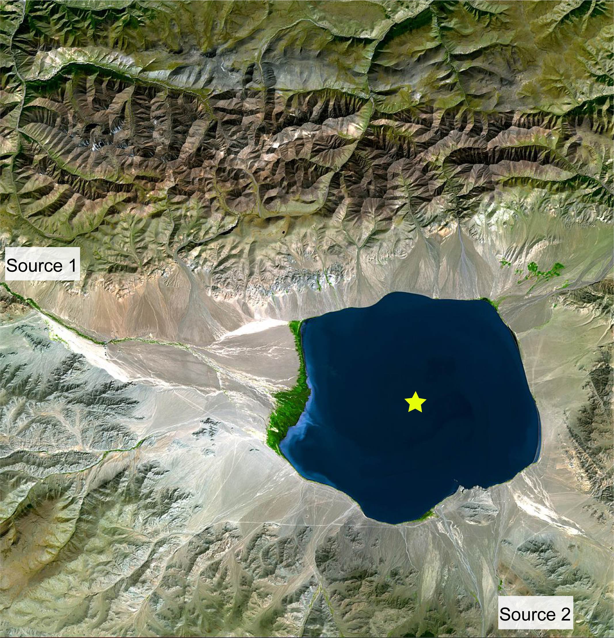
Google Earth image for exercise 3.8 showing where the sediment was collected. — Figure 3.25 – Google Earth image for Exercise 3.8. The yellow star is the location where the sediment was collected. The two potential sources are labeled.

You collect five biotite grains from Source 1, five biotite grains from Source 2, and measure them using the potassium-40 system. What are the ages of these source-rock biotite grains? Fill this out in Table 3.7.

Table 3.7 – Worksheet for Exercise 3.8a
Samples from Source 1	Parent : Daughter	Age
1a	1 : 0.808
1b	2 : 1.706
1c	1 : 0.825
1d	3 : 2.349
1e	2 : 1.596
Samples from Source 2	Parent : Daughter	Age
2a	2 : 0.626
2b	4 : 1.236
2c	1 : 0.323
2d	3 : 0.903
2e	2 : 0.596

What is the average age of the rocks at Source 1? _______________
What is the average age of the rocks at Source 2? _______________

The lake sediment grains you collected have the following ages. Determine which source area they most likely came from by filling out Table 3.8.

Table 3.8 – Worksheet for Exercise 3.8d
Lake Sediment	Age	Source Area
1	523 Ma
2	1,157 Ma
3	517 Ma
4	521 Ma
5	486 Ma
6	1,116 Ma
7	513 Ma
8	501 Ma
9	523 Ma
10	494 Ma

What percentage of the lake sediment is coming from Source 1? _______________
What percentage of the lake sediment is coming from Source 2? _______________
Critical Thinking: What could be the reason(s) why you see this sediment distribution in the lake?

Exercise 3.9 – Using Principles of Relative Dating on Other Planets

Cross-cutting relationships is a universal principle. That means it not only applies to our planet but applies to other planets. Let’s take a look at some pictures taken from the surface of Mars; these show features such as craters, rivers, and fractures (a type of fault). These types of images are used to decipher the tectonic, volcanic, and impact history.

Look at Figure 3.26.
1. Which is older, Crater B or Crater S? ____________________
2. Explain why.
3. Which is older, Fracture F or Crater B? ____________________
4. Which is older, Fracture F or Crater S? ____________________
5. Critical Thinking: If you wanted to land a rover to investigate Crater B, where would it be safe to land? Consider whether or not you think Fracture F is an active fault.
  
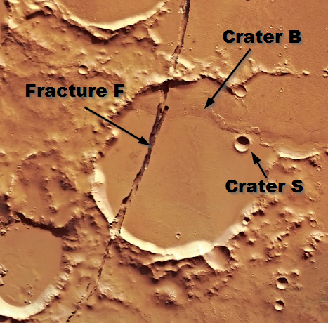
  $Martian craters and fractures for exercise 3.9a$
  Figure 3.26 – Image for Exercise 3.9a. Martian craters near Cerberus Fossae in the Elysium Planitia region close to the Martian equator. Photo taken January 2018. Image credit: Adapted from ESA/DLR/FU Berlin, CC BY-SA IGO.
Look at Figure 3.27. Put the craters in relative order from oldest to youngest. ______________________________

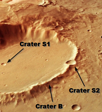
Figure 3.27 – Image of Hadley crater for Exercise 3.9b. This is a composite of several images taken during revolution 10572 on 9 April 2012 by ESA’s Mars Express centered around 19°S and 157°E; the image has a ground resolution of about 19 m per pixel. The image shows the main 120 km wide crater, with subsequent impacts within it. Evidence of these subsequent impacts occurring over large time scales is shown by some of the craters being buried. This image shows one of the characteristics of Martian craters as they often have fluidized ejecta that can be seen both in the bottom right and top left craters, the latter crater reaching a depth of around 2600 m. Image credit: Adapted from ESA/DLR/FU Berlin, CC BY-SA IGO.
Look at Figure 3.28.
1. Which is older, Crater C1 or River R1? ____________________
2. Which is older, Crater C2 or River R2? ____________________
  
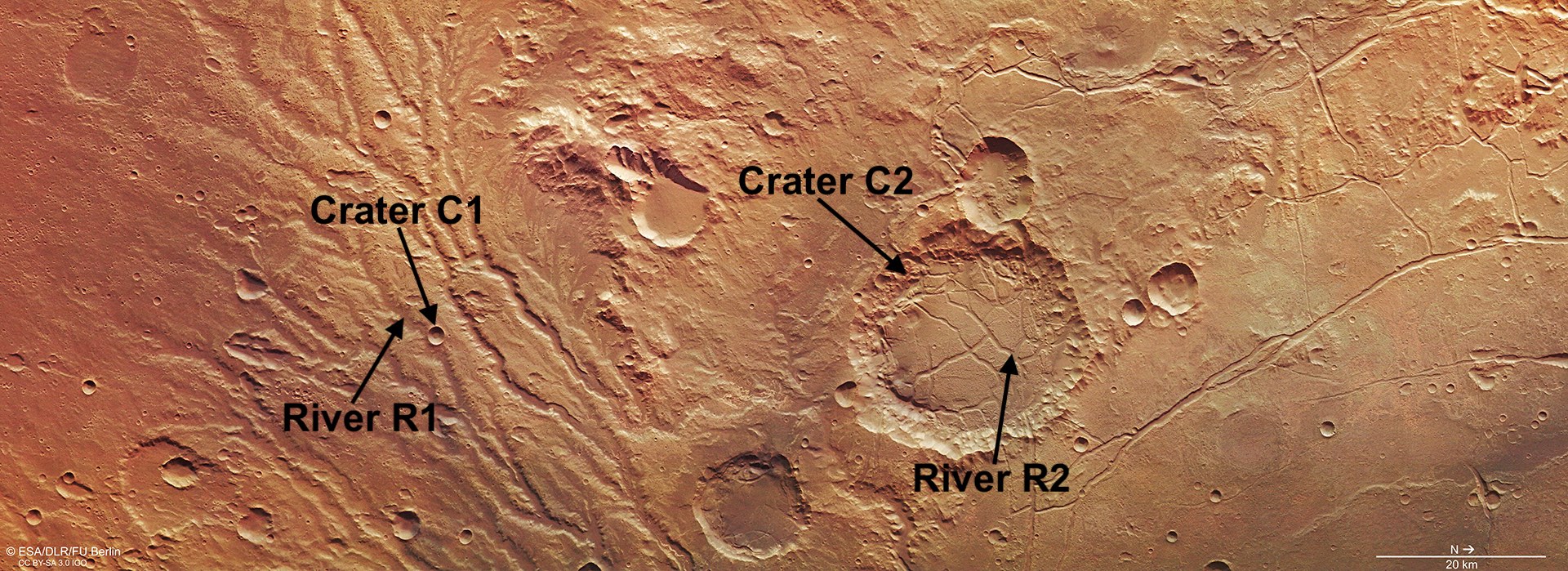
  Figure 3.28 – Image from the Arda Valles region of the Martian highlands for Exercise 3.9c. The region was imaged by Mars Express on 20 July 2015 during orbit 14649. The image is centered on 19°S / 327°E; the ground resolution is about 14 m per pixel. Image credit: Adapted from ESA/DLR/FU Berlin, CC BY-SA IGO.