
Chapter 11: Paleoclimate
The 2nd edition is now available! Click here.
Learning Objectives
The goals of this chapter are to:
- Understand the different sources of evidence used to study past climates
- Recognize the processes influencing natural climate change
- Use geologic evidence to interpret past climates
11.1 Introduction
Earth’s climate has constantly changed throughout its existence, with periods that have been much warmer and cooler than today. Evidence of these climate variations is found in the geologic and fossil records, and geologists use them to interpret how climate has changed through time. The study of past climates is called paleoclimatology.
Geologists can’t directly observe past climates because they already happened; no temperature or precipitation can be measured. Instead, geologists turn to the geologic record to study things dependent on climate, in a sort of second-hand view. These secondary sources of information are called proxies. The most common proxies used to interpret past climate are fossils, but ice cores, tree rings, and sediment cores are also used. For example, a particular species of foraminifera coils its shell (technically called a test) to the left or right, depending on whether the seawater temperature was cooler or warmer. While this does not give an exact temperature, it gives you a relative idea of the conditions. If you were to find mostly right-coiling fossils in a layer of sediment, you would know that seawater temperature was relatively warm during the time those organisms lived.
Exercise 11.1 – Foram Morphology as a Climate Signal
Foram fossils are an excellent proxy for paleoclimate because their growth is influenced by climate and ocean conditions. Some species of foraminifera are so sensitive to seawater temperature that they will alter the way they grow their test (hard shell). Neogloboquadrina pachyderma, for example, is a species of planktonic foraminifera that will coil its test to the right when ocean water is warmer and coil to the left when ocean water is cooler.
In a sediment core recovered from the North Atlantic Ocean, you counted the number of left- and right-coiling varieties of N. pachyderma to help interpret paleoclimate for the past 160,000 years. Samples of the sediment core were taken at 10,000-year intervals.
- Complete Table 11.1 by calculating the values for the total number of N. pachyderma for each sample, the percentage of the right-coiling variety, and the percentage of the left-coiling variety. The first row is done for you.
Table 11.1 – Worksheet for Exercise 11.1 Age (years ago) Right-coiling N. pachyderma Left-coiling N. pachyderma Total number N. pachyderma % Right-coiling N. pachyderma % Left-coiling N. pachyderma 0
230 50 280 82% 18% 10,000 220 75 20,000 70 230 30,000 45 300 40,000 50 302 50,000 65 389 60,000 20 140 70,000 56 287 80,000 63 267 90,000 212 56 100,000 120 23 110,000 87 45 120,000 203 66 130,000 56 205 140,000 45 332 150,000 89 135 160,000 123 166 - Plot the percentage of right-coiling N. pachyderma on the blank graph in Figure 11.1 (or make your own graph in Microsoft Excel). The x-axis is the percent of the right coiling variety, and the y-axis is the age of the sediment sample the forams were in.
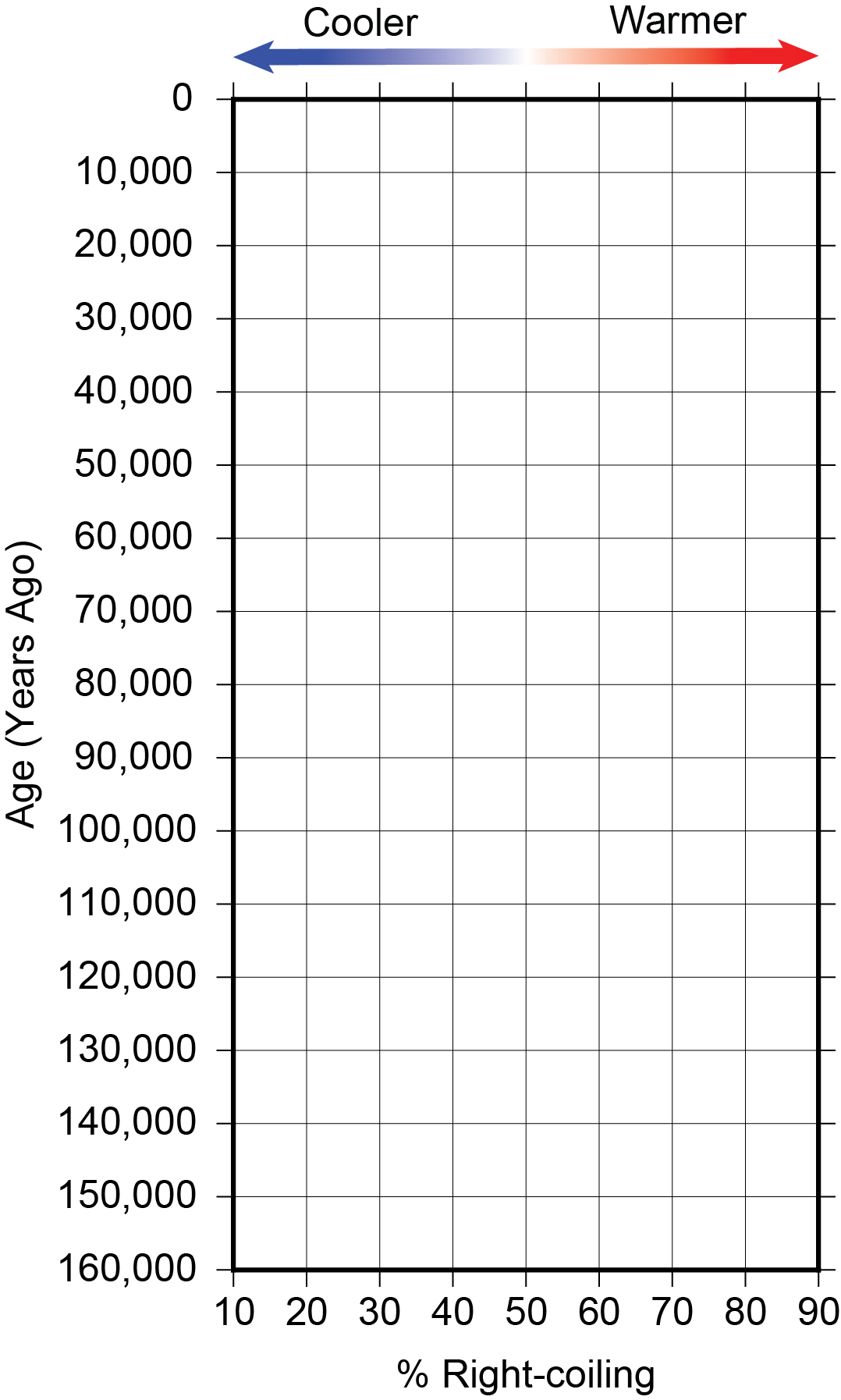
Figure 11.1 – Graph for Exercise 11.1. - Has climate changed in the last 160,000 years?
- On your graph in Figure 11.1, indicate where warm and cold periods occur.
- How many times has it been warm with a high percentage of right coiling forams? You should group several points as one time interval. For example, you could group 0 and 10,000 years as one time interval.
- Has the length of time that it has been cool (with a low percentage of right coiling forams) been the same each time there has been an ice age?
- Why does the total number of forams vary between samples? Does the number of forams vary with climate?
- Critical Thinking: How does the length of time of the ice ages compare to the length of time it was hot? Can you think of a reason for this difference?
Exercise adapted from Hilary Clement Olson, Learning from the Fossil Record.
11.2 Causes of Natural Climate Change
Climate change is complex, and many factors affect Earth’s climate system. These include Earth’s orbital patterns, plate tectonics and the position of continents, changes in solar output, changes in atmospheric greenhouse gases, and others. All operate at various time scales that alter Earth’s climate over hundreds, thousands, and millions of years.
On a time scale of millions of years, the movement and location of continents is the biggest influence on Earth’s climate system. The position of continents affects ocean and atmospheric circulation, which are the two conveyor belts responsible for taking excess heat from the equatorial regions and moving it to the polar regions.
On time scales of thousands to hundreds of thousands of years, Earth’s orbital patterns have the greatest effect on climate. Earth’s orbit varies on three different cycles, called Milankovitch cycles. The shape of Earth’s orbital path around the sun changes from more circular to more elliptical, completing an entire cycle about every 100,00 years. This is known as eccentricity. Eccentricity changes how close Earth is to the sun, affecting how much solar radiation the planet receives.
Earth has a tilt to its axis, and it moves back and forth between 22.1 and 24.5 degrees. This cycle, known as obliquity, takes about 41,000 years. Obliquity changes increase seasonality when the angle is higher and decrease seasonality when the angle is lower. Seasonality refers to the difference between summer and winter temperatures. Higher seasonality means hotter summers and colder winters; decreased seasonality means mild summers and mild winters.
The last orbital change is called precession, best described as a wobble around Earth’s axis. If you’ve ever spun a toy top as a kid, you may remember that as the top slows down, it begins to wobble. That wobble is the same as Earth’s precessional cycle, which takes nearly 26,000 years. Precession affects the timing of seasons because it changes what time of year the northern hemisphere points toward the sun. Today, the northern hemisphere experiences summer during June-September, but in 13,000 years, the northern hemisphere will have winter during those months.
These three cycles can work together to amplify climate change or work against each other to dampen it. They also have much longer versions that affect climate on longer time scales. For example, eccentricity also has 400,000-year and 2.4 million-year cycles and obliquity has a 1.2 million-year cycle.
It’s important to note that these natural causes of climate change cannot explain the magnitude of warming and climate change that we see happening today. Current climate change can only be explained by human influences, particularly from the release of greenhouse gases from burning fossil fuels.
11.3 Oxygen Isotopes as a Climate Proxy
There are many ways fossils can be used as proxies. One of the most common uses is stable oxygen isotopes in organisms like forams and diatoms. Forams and diatoms are shelled organisms found in aquatic and marine environments. There are both planktonic forms floating in the water column, benthic forms that are bottom-dwellers. Foram shells are made up of calcium carbonate (CaCO3), while diatom shells are composed of silicon dioxide (SiO2). Do these formulas look familiar? They are essentially calcite and quartz. These organisms extract these elements from the seawater to build their shells. Oxygen, in particular, is sensitive to global climate and has different isotopes that vary in abundance based on how much ice is on the planet.
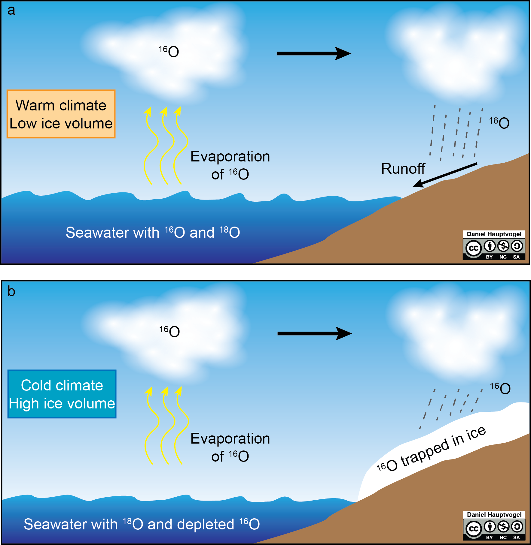
Oxygen-16 (16O) is the most common form of oxygen, with 8 protons and 8 neutrons. Oxygen-18 (18O) is less abundant but has two extra neutrons, making it slightly heavier than 16O. Since 16O is lighter, water molecules containing it are preferentially evaporated from the oceans than its heavier counterpart (18O is evaporated too but in smaller quantities, Figure 11.2). When the water vapor begins to condense into rain or snow, heavier 18O isotopes preferentially do so. The remaining water vapor then has even less 18O. If temperatures in the polar regions are cold enough when precipitation falls, the water turns to snow and ice and becomes stuck on the continent in ice sheets instead of flowing back to the ocean. This is important because, during cold times, oceans become relatively enriched in 18O because 16O is being extracted and stored on continents in the ice. When these organisms build their shells, the chemistry of the shell reflects the chemistry of the seawater. Suppose you have a sediment core containing an abundance of these organisms. In that case, you can look at their shell chemistry for changes in 18O to interpret how much ice was on that planet.
Exercise 11.2 – Using Oxygen Isotopes to Interpret Climate
One of the most famous oxygen isotope records in paleoclimatology is from Drs. Lorraine Lisiecki and Maureen Raymo, who published an extremely detailed record of the past 5.3 myrs from foraminifera. Figure 11.3 is a portion of this oxygen isotope record that spans the last 800 kyrs. The notation used for oxygen isotope records is δ18O (usually pronounced as delta-O-eighteen), which is the ratio of 18O to 16O. The higher the number, the more 18O there is. The unit is per mil (‰), which looks like a percent sign with an extra 0 in the denominator because it is out of a thousand instead of a hundred.
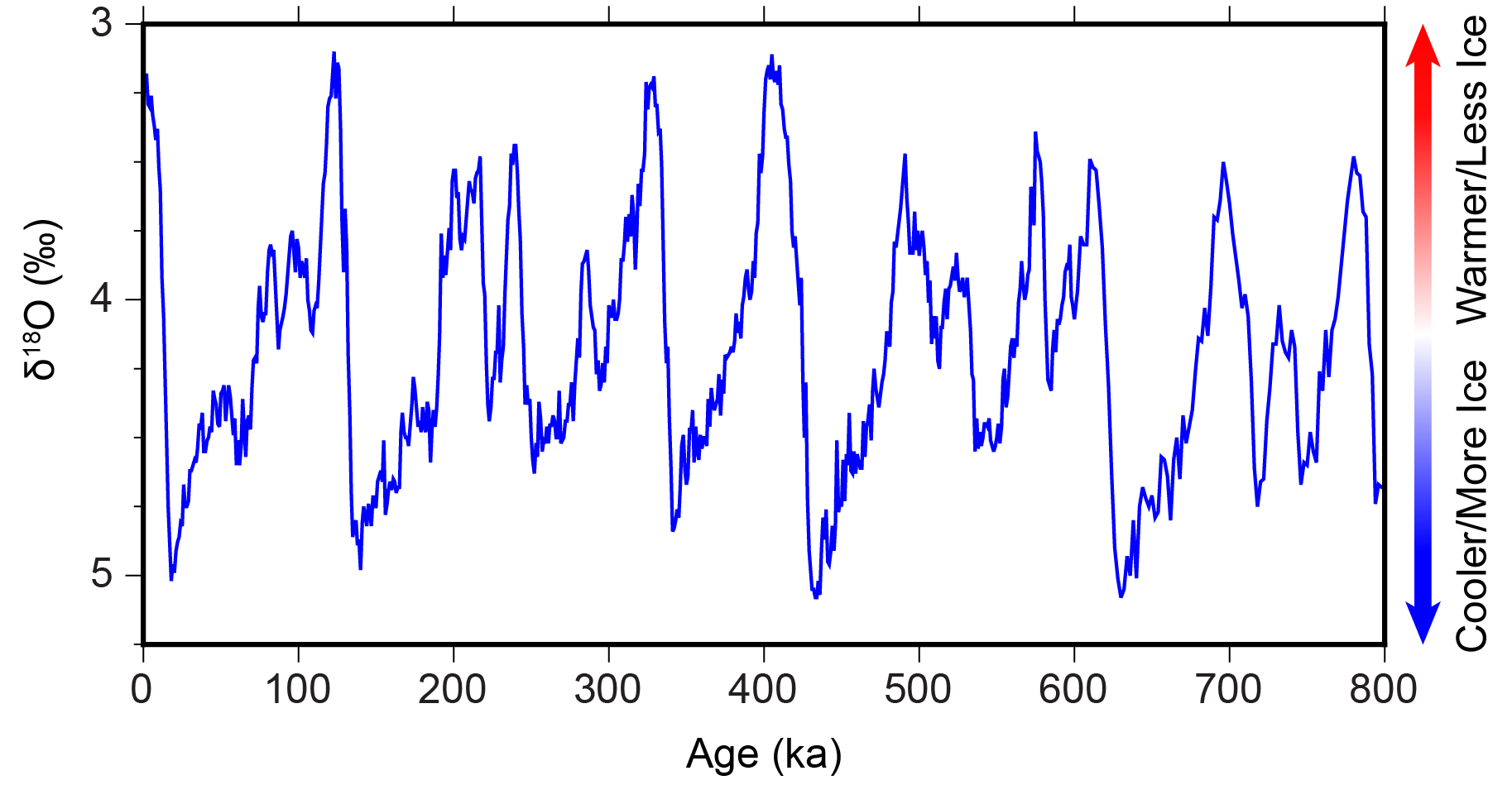
- How many distinct cold periods can you identify in Figure 11.3? ____________________
- About how far apart are these cold periods? ____________________
- What do you think has been controlling natural climate change over the past 800,000 years? Explain.
- Compare and contrast the transitions from warm to cold periods and from cold to warm periods.
- Critical Thinking: If we assume that much of this oxygen isotope signal is a proxy for ice volume, do you think it takes longer for ice sheets to grow or melt? Explain.
Exercise 11.3 – The Climate Record of the Past 65 myr
For Earth’s climate record, we know the most about the past 65 myr than we do for the rest of Earth’s history. Figure 11.4 contains oxygen isotope and sea-level data for the entire Cenozoic.
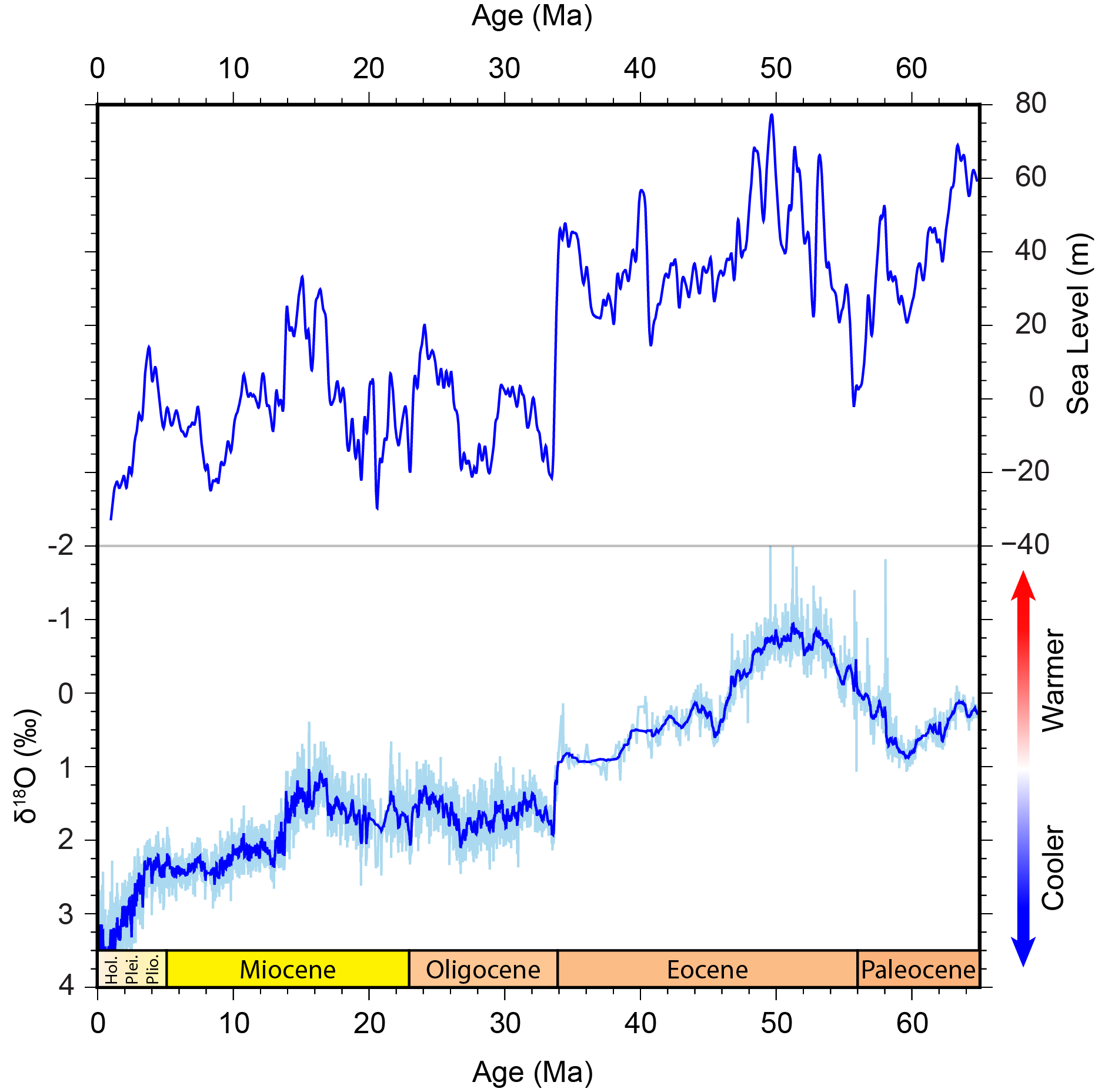
- Table 11.2 contains major climate events of the past 65 myr. Identify these events in Figure 11.4.
- Explain why there is a steep drop in sea level during the Eocene-Oligocene transition.
| Event | Description |
| Paleocene-Eocene Thermal Maximum (PETM) | A short, 200,000 year period where massive amounts of carbon dioxide were released into the atmosphere, and global temperatures increased by 5-8 °C. |
| Early Eocene Climatic Optimum (EECO) | A 2 myr period of the warmest temperatures of the past 65 myr. |
| Late Eocene Cooling | A global cooling driven by lowering CO2. |
| Eocene-Oligocene Transition | Permanent ice sheets form in Antarctica, driven by CO2 lowering past a critical threshold and changes in ocean circulation from moving continents. |
| Middle Miocene Climatic Optimum (MMCO) | A prolonged warm period whose cause is still debated. |
| Middle Miocene Climate Transition (MMCT) | Antarctic ice sheet expansion and global cooling driven by lower CO2 and changes in ocean circulation. |
| Pleistocene Glaciations | Repeated glacial cycles in which northern hemisphere continental glaciers reached as far south as 40° latitude. |
11.4 Tree Rings as a Climate Proxy
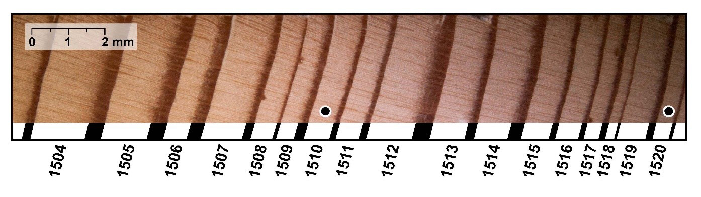
Every year, trees grow taller, and their trunks grow wider. The new growth that makes the trunk wider is called a tree ring. Tree rings are a valuable tool to climate scientists because they contain a record of temperature and precipitation. During dry years, trees hardly grow at all and create narrow rings. However, during rainy years, trees will grow more than usual and have wide rings. Because of this difference in ring size and connection with precipitation, scientists can use tree ring patterns to learn about the climate during the time the tree lived. The science of studying tree rings to see what they tell us about past climates is called dendrochronology.
Each tree ring has a wider light-colored portion and a narrow dark-colored portion (Figure 11.5). The light coloring, called the earlywood, forms during the winter and early spring precipitation as trees grow at their greatest rate. The darker color, called the latewood, forms in late summer during slower growth in anticipation of the dormant season to come. A full year’s growth includes both a light, earlywood ring and a dark, latewood ring. Together, they make up one tree ring.
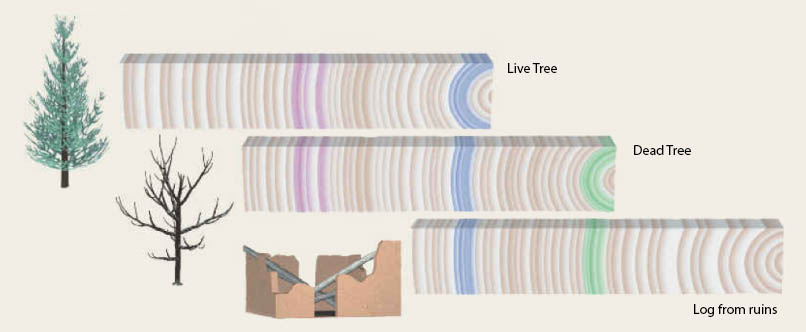
Data from multiple trees can be combined to create a longer history than a single tree can make. To do this, dendrochronologists match patterns in the rings from each tree (Figure 11.6). For example, if tree A started growing in 1830 and died in 1930, and tree B started growing in 1910 and died in 2010, scientists can combine the records of both trees by matching the patterns for the 20 years that both trees lived. Dendrochronologists rarely cut down trees to analyze rings. Instead, they take a thin coring tool to extract a core about the thickness of a pencil without harming the tree.
Exercise 11.4 – Investigating Tree Ring Growth and Climate
You have been given four simulated tree ring cores (Figure 11.7) from the following sources:
- Core Sample 1: From a living tree from the Pinetown Forest in the fall of 2018
- Core Sample 2: From a tree from the Pinetown Christmas Tree Farm a few years ago
- Core Sample 3: From a log found near the main trail in Pinetown Forest
- Core Sample 4: From a barn beam removed from Pinetown Hollow
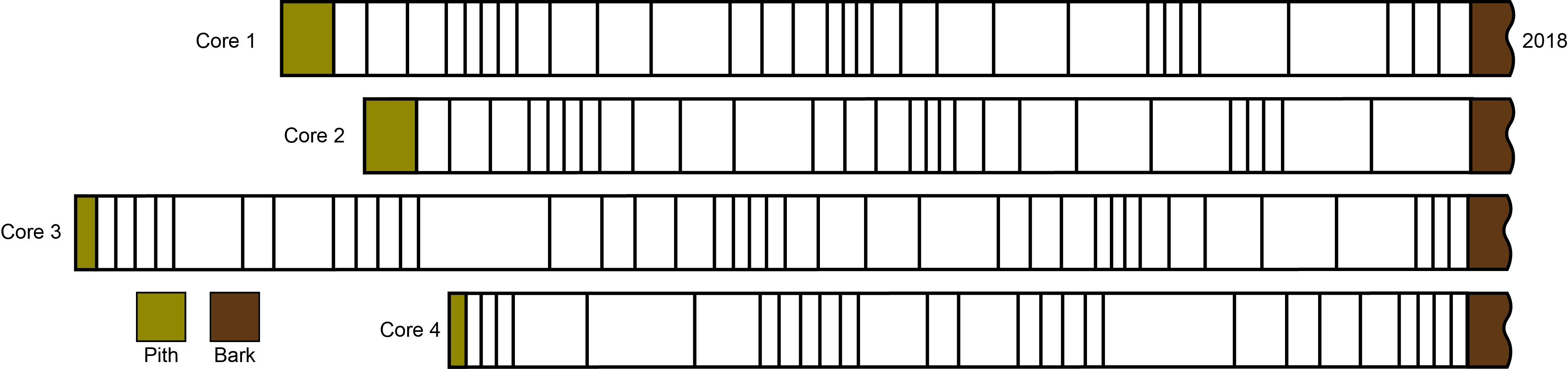
- Count the number of tree rings in each core sample. That number is the age of the tree in years. Record the ages in Table 11.3. Don’t count the pith, which is a special plant tissue found at the center of tree trunks.
- Determine the year that tree from core sample 1 started growing. Fill this out in Table 11.3.
- Cut out the 4 tree ring records. Match the patterns in core sample 1 and core sample 2 by lining up the records and looking at what years overlap in both records. Determine when the tree from core sample 2 started growing and when it was cut/cored.
- Follow the same steps for core sample 3 and core sample 4.
Table 11.3 – Worksheet for Exercise 11.4 Core Sample Age of Tree Year Growth Began Year Cut or Cored 1 2018 2 3 4 - Which tree ring matches the year you were born? ____________________
- Was the weather in Pinetown the year you were born good for tree growth or not? Explain.
- Over the entire record, how many years were good for tree growth, and how many were not?
11.5 Fossils as a Climate Proxy
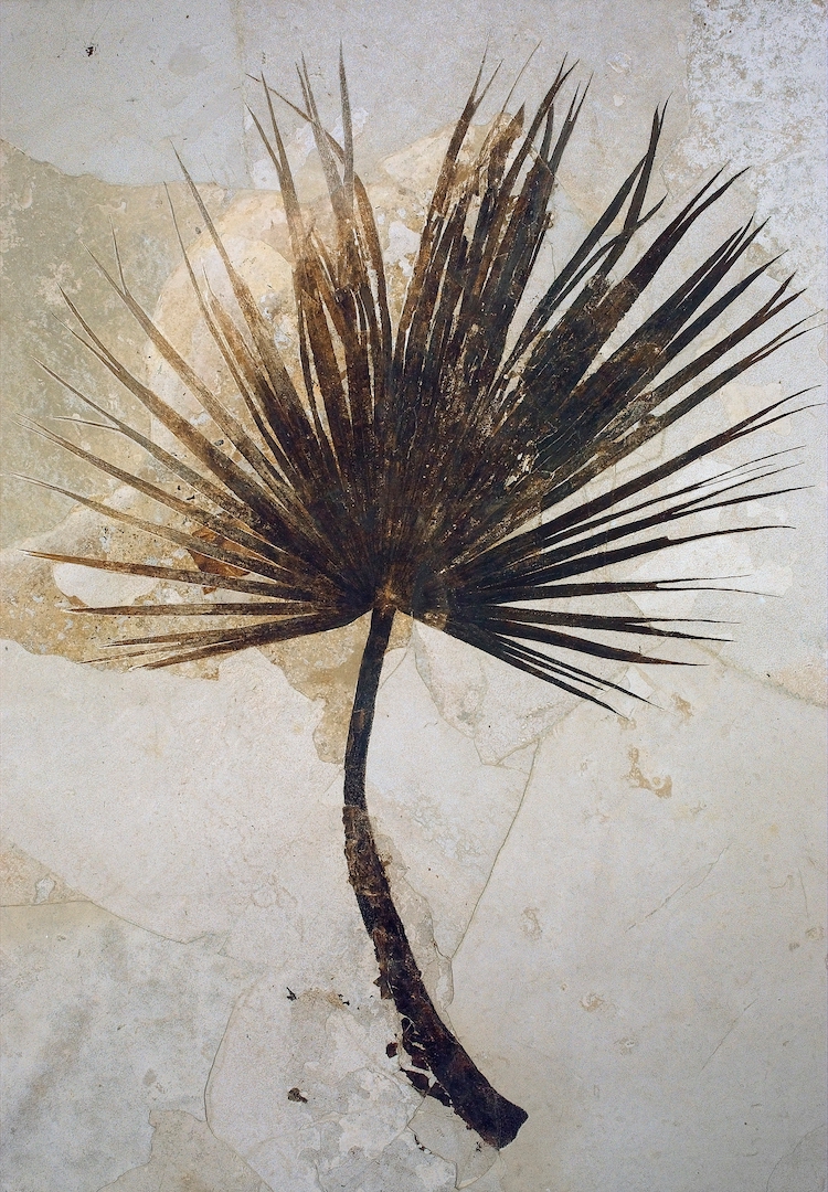
The foraminifera fossils used to construct oxygen isotope records are not the only use of fossils for paleoclimate. Many fossils in the geologic record can provide at least some information about climate. For example, fossils of palm trees from the Green River Formation in Wyoming (Figure 11.8) suggest climate there was subtropical during part of the Eocene 50 Mya, similar to what Florida is like today. If you look at the oxygen isotope record for the past 65 myr in Figure 11.4, you’ll notice that at 50 Ma, we had the warmest climate of the Cenozoic. This is an excellent example of using multiple sets of data to support ideas in science.
Pollen fossils are widely used to interpret paleoclimate. Pollen grains (Figure 11.9) have a resistant outer shell that helps to keep them preserved in the geologic record, and they are very common. The study of pollen is called palynology, and palynologists use these fossils from sedimentary records to interpret what climate was like. Each plant species produces a different sized and shaped pollen grain, and palynologists can determine which type of plants were present or trace the migration of plants as climate changes.

Exercise 11.5 – Using Fossil Pollen to Track Ice Sheet Movement

During the late Quaternary, our planet experienced large, rapid changes in climate associated with the growth and retreat of continental ice sheets. These changes were related to major reorganizations of terrestrial habitats, especially in the northern hemisphere. Ice age mammals like the classic mammoths and mastodons had to cope with these changes, as did our own species, Homo sapiens, as we expanded out of Africa during this time.
Because plant and animals species often have specific climate requirements, we can use the geographic distribution of fossil species to reconstruct ancient climate parameters and document how these parameters changed over time. The coniferous tree species Picea mariana (Figure 11.10) and Picea glauca, commonly known as black spruce and white spruce, are the two most abundant and widely distributed Picea species in North America. Their migration with changing climate is well-documented through pollen fossils. Their modern habitat, like all spruces, is in boreal forests or mountains, most commonly found in Canada and some parts of the northern U.S.
Part 1
You will document the modern distribution of Picea mariana and its preferred climate conditions.
- Take a close look at Figure 11.11. In terms of geography, what is the extent of Picea mariana’s habitat?
- Figure 11.11 also shows Picea mariana’s modern temperature and precipitation ranges. Describe the type of climate this tree grows in.
- Predict how the distribution of this tree taxon has changed over the last 21,000 years. Do you think it has remained in the same position, or has it migrated through time?

Part 2
In this part, you will look at the distribution of all Picea species over time using the Neotoma Database, which will show you the locations where its pollen grains have been found. The Neotoma database is a repository for paleoenvironmental data, including pollen fossils.
Follow these steps:
- Go to the Neotoma Database and click on the Explorer icon. The search window should automatically pop up; if it doesn’t, click on the binoculars icon.
- For dataset type, select “pollen” from the dropdown menu.
- Click on the gears symbol next to the “Taxon name” box and select “vascular plants” from the Taxa group pull-down menu.
- In the “Search for” box, type “Picea” and click “Go”.
- Select all species of Picea and click close (We are using all species because not all scientific studies have separated Picea fossils into different species. Instead, they simply reported the fossil as Picea sp. There are only a few species of Picea in North America, and their habitats and climate conditions are similar in boreal forests or mountainous areas.)
- Click the checkbox next to “Abundance/density” and set the abundance to “> 20%”.
- Click on time and set the age range to 21,000 (oldest) to 18,000 (youngest) and hit search.
After a few seconds, your map will update with the locations of pollen fossils for Picea sp. at the indicated time range.
- Where in North America did Picea sp. exist? How does that compare to the modern distribution of Picea mariana?
- Based on the modern climate conditions and habitat for Picea, what was the climate like for the U.S. during this time?
Repeat the search for the following time ranges; you will only need to change the time range, all other options should not have to be selected again:
- 15,000 to 12,000 yr BP
- 10,000 to 7,000 yr BP
- 5,000 to 1,000 yr BP
Observe the patterns for spruce at each time slice on the map. You can change the symbols and colors, rearrange the plotting order, and turn layers on and off using the View Current Search Layers tool (it’s next to the binoculars icon)
- Describe the distribution of Picea sp. through time.
- What climate parameter (temperature or precipitation) do you think is driving the distribution of Picea through time? Explain your reasoning.
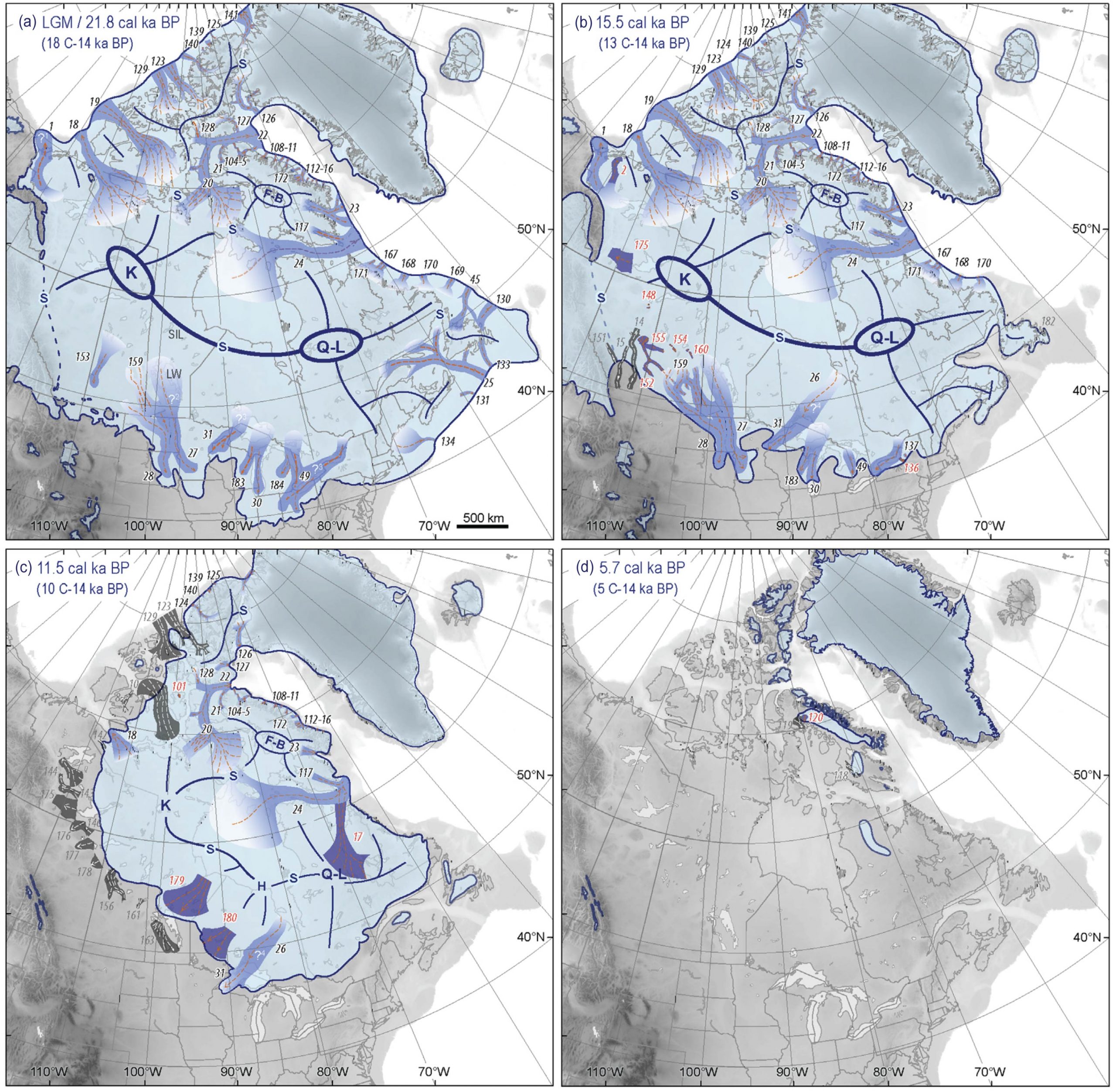
- Compare the distribution of Picea through time to the location and size of the Laurentide Ice Sheet in Figure 11.12. How does the position of Picea relate to the position of the ice sheets?
- Critical Thinking: This exercise focused on one species of a conifer. Most conifers are restricted to either high elevation or high latitudes. What types of trees could you use for tracking glacial history in temperate or tropical locations?
This exercise was adapted from Samantha Kaplan, Margaret Yacobucci, and John Williams.
11.6 Sediment as a Climate Proxy
Sediment on the continent or at the bottom of the ocean can give geologists a lot of information about what the climate was like when sediment was deposited. Not only does that sediment contain fossils that provide clues, but the grain size and provenance of the sediment can help determine temperature and precipitation patterns. In polar regions, geologists can use the sedimentary record to determine how far ice sheets advanced and when they retreated. Those IODP Expeditions we talked about in Chapter 5 are among the primary ways sedimentologists study past climates.
Exercise 11.6 – Using Sediment Provenance to Determine Paleoclimate in Antarctica
All rocks have a distinct chemical makeup; even rocks of the same type can have slight variations. When sediment is weathered and eroded from rocks, the sediment retains this chemical makeup. Thus, when geologists recover sediment, like drilling a sediment core from the ocean floor, they can analyze the sediment chemistry and match it up with known sources on the continent.
Ice sheets are large ice masses that sit on top of continents. Antarctica, for example, is a continent a bit larger than the U.S., and 98% of it is covered by an ice sheet that is two to three miles high. Ice on continents flows, like water flowing through a series of rivers but at a much slower pace. As the ice moves across the rocky surface, it weathers and erodes sediment. Most of this erosion occurs at the edge of the ice sheet, where the ice is moving fastest. When ice sheets reach the coastline, the sediment is then carried by ocean currents to eventually be deposited. When geologists investigate sediment eroded by glaciers, they can use the geochemical fingerprint of the sediment, match it to rocks that exist on the continent, and determine where the edge of the ice was because that is where the most erosion was taking place.
Figure 11.13 is a map of Antarctica with a focus on a region called the Wilkes Subglacial Basin. A marine sediment drill core was taken from a location just off the coast; the site is labeled U1361A. Layers of sediment recovered from this core were analyzed for two trace element geochemical signals, neodymium (Nd) and strontium (Sr). These trace elements have several uses in geology, but we will use them as indicators of provenance.
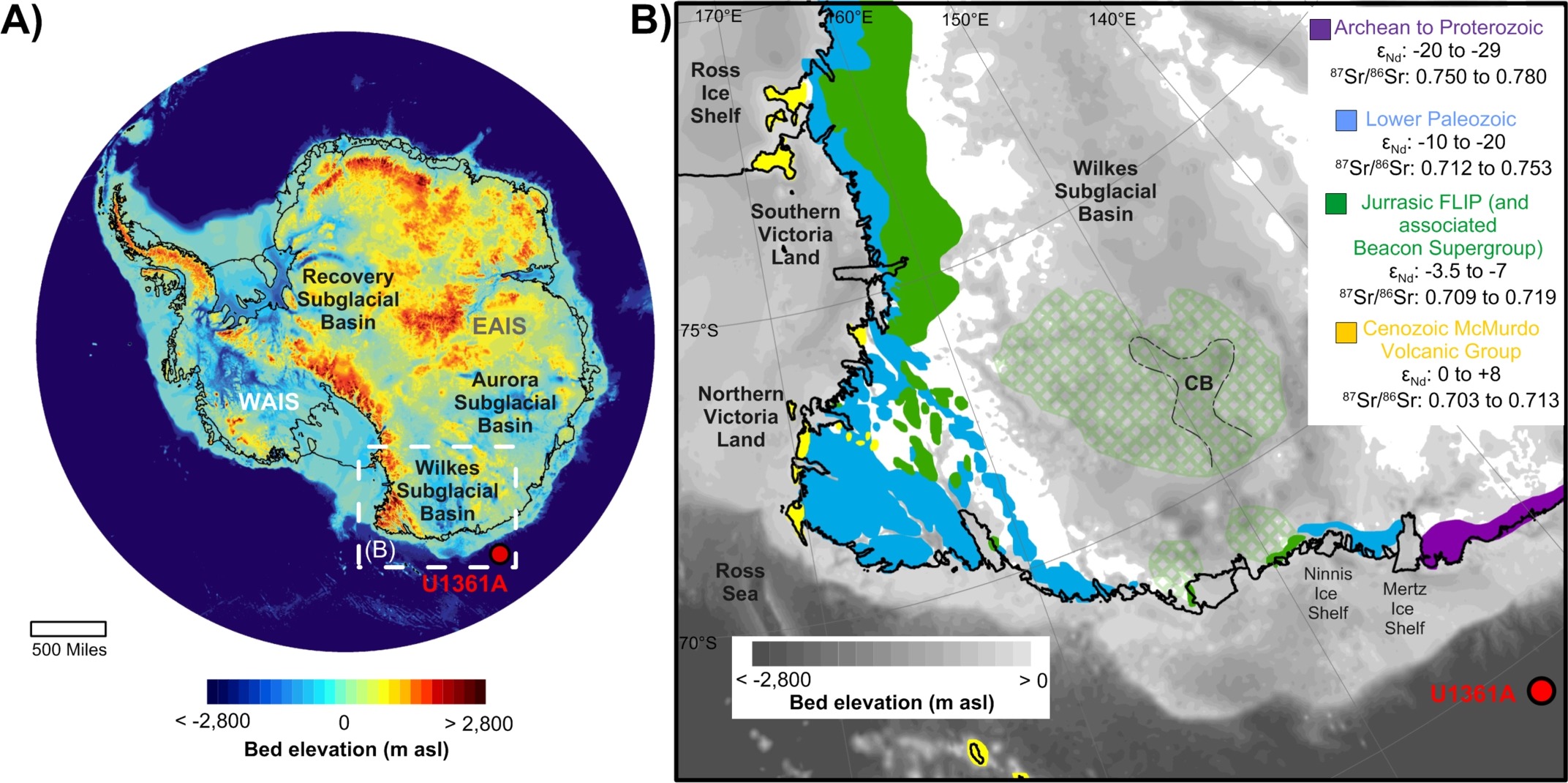
Figure 11.14 contains five different types of data collected from the layers of sediment in this core: sediment type, natural gamma radiation, diatom concentration, Sr, and Nd. Diatoms are single-celled, photosynthetic algae that build a body out of silica. Generally speaking, diatoms are more productive when water temperature increases. Use these data sets to answer the following questions.
- Describe any trends or patterns that you can see in the data in Figure 11.14.
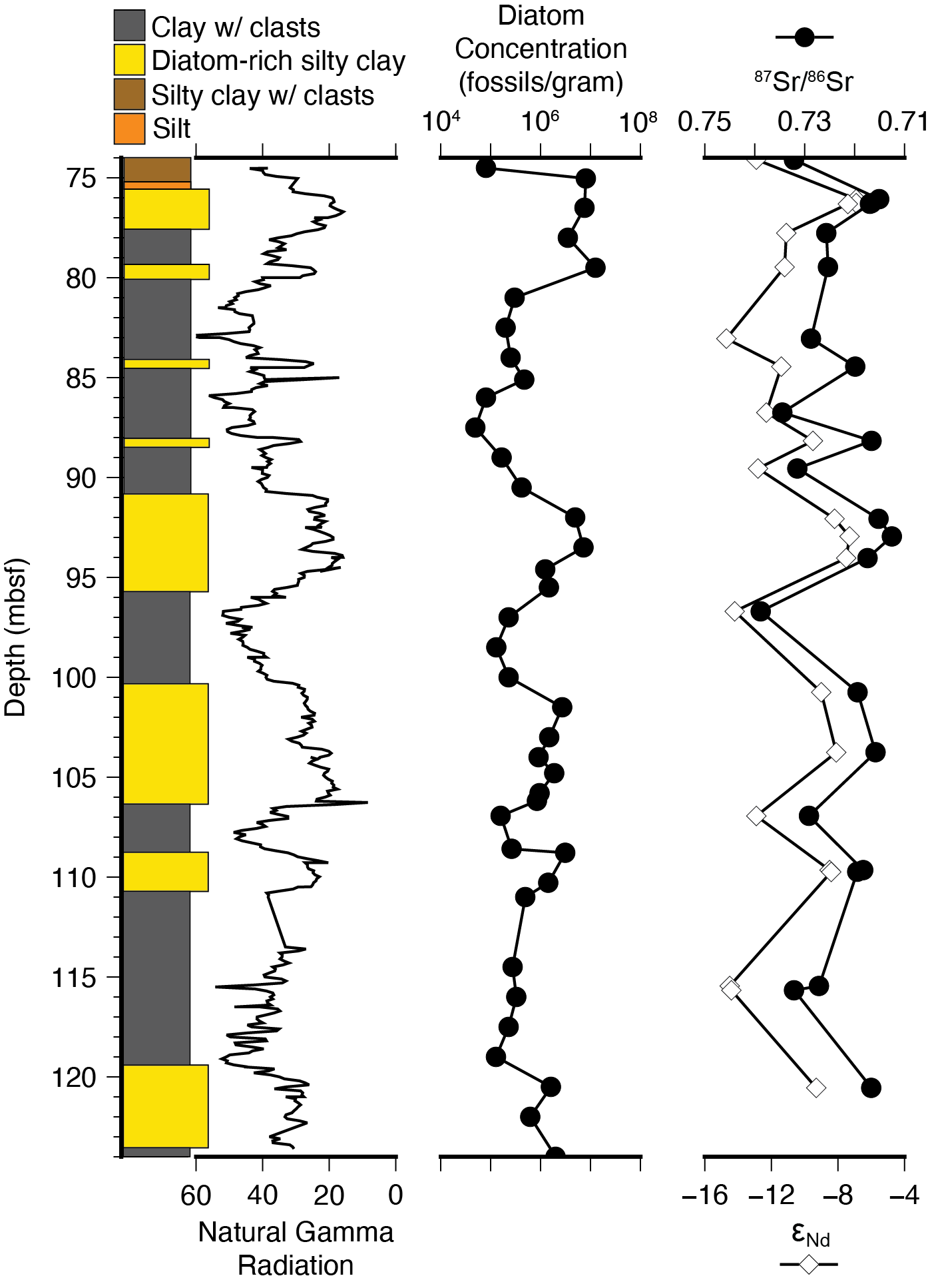
Figure 11.14 – Lithostratigraphy (Escutia et al., 2011), natural gamma radiation, diatom valve concentrations, and Nd and Sr isotopic compositions from Site U1361A. Lithostratigraphy and natural gamma radiation are from Escutia et al. (2011), diatom, Nd, and Sr data are from Cook et al. (2013). mbsf = meters below seafloor. Image credit: Daniel Hauptvogel, CC BY-NC-SA. - Table 11.4 contains the Sr and Nd chemical analyses collected from sediment in the drill core (the same data is plotted in Figure 11.14). Using Figure 11.14, note whether each Sr and Nd analysis was from diatom-rich or diatom-poor layers.
Table 11.4 – Sr and Nd isotopic data Depth (mbsf) 87Sr/86Sr εNd Diatom-rich or Diatom-poor 74.09 0.73215 -12.9 76.07 0.715075 -6.9 76.27 0.716604 -6.9 76.31 0.716901 -7.4 77.77 0.72563 -11.1 79.47 0.725313 -11.2 83.05 0.72871 -14.7 84.45 0.71985 -11.4 86.75 0.734461 -12.3 88.17 0.716557 -9.5 89.55 0.731468 -12.8 92.07 0.715194 -8.2 92.95 0.712514 -7.3 94.03 0.717386 -7.5 96.7 0.738815 -14.2 100.75 0.719381 -9 103.76 0.715787 -8.1 106.94 0.729142 -12.9 109.65 0.718272 -8.5 109.74 0.71947 -8.4 115.45 0.72711 -14.5 115.67 0.732095 -14.4 120.55 0.716649 -9.3 - Figure 11.15 is a graph comparing Sr and Nd values for the four potential source areas of the sediment, with colors matching the areas from the regional map in Figure 11.13. Plot the Sr and Nd data on this graph using different colors/shapes for samples from diatom-rich and diatom-poor layers.
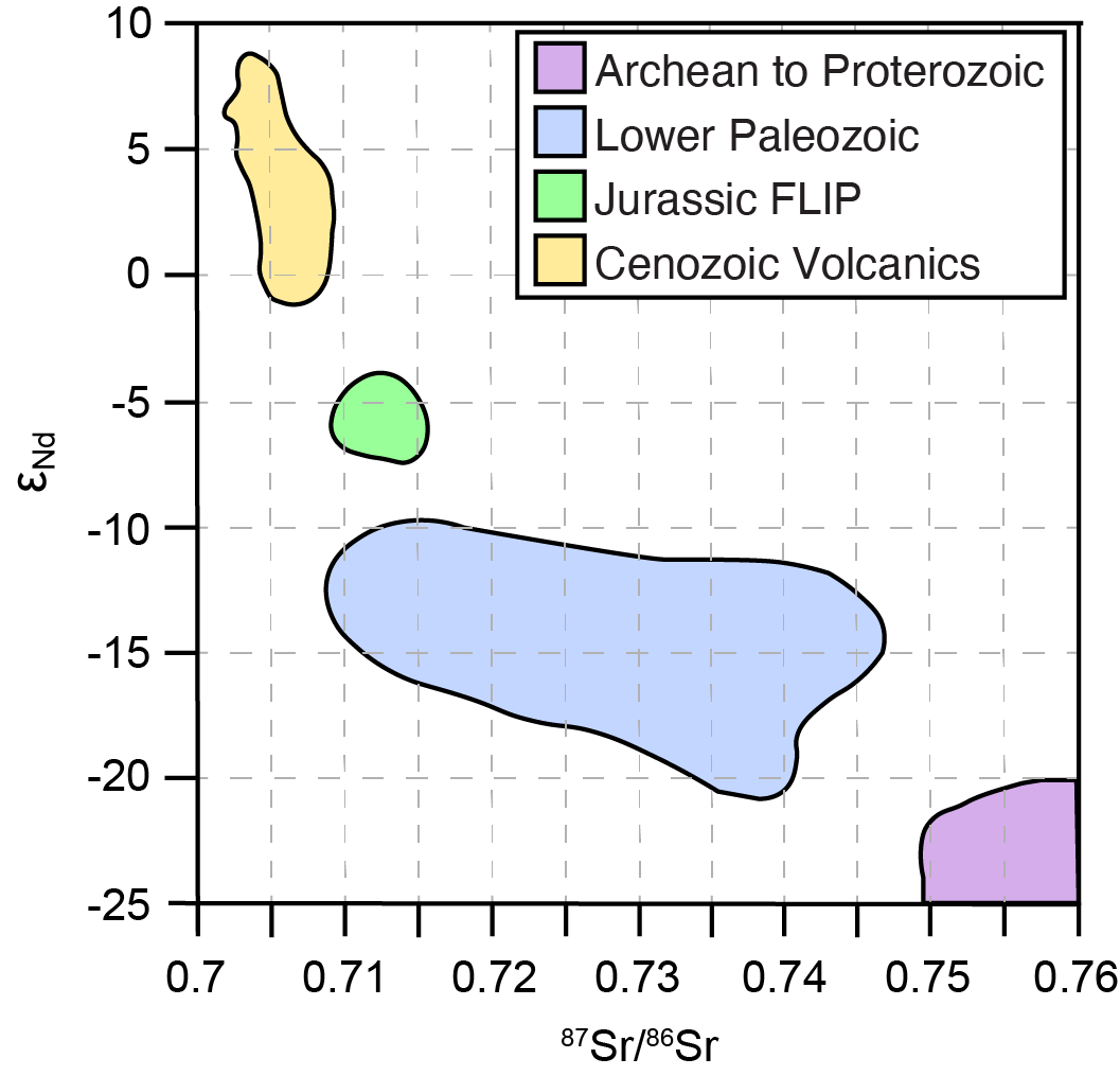
Figure 11.15 – Characteristic geochemical signatures of the different lithological terranes in the Wilkes Subglacial Basin vicinity. Image credit: Daniel Hauptvogel, CC BY-NC-SA, adapted from Bertram et al. (2018). - Why do some of the samples plot inside the known chemistry of potential source areas (the colored polygons) and some plot outside of them?
- Which source(s) are primarily contributing sediment to Site U1361A? ________________________________________
- When the edge of the ice sheet retreats inland, which source area should become more abundant? ____________________
- Combining all the data, explain whether diatom-rich or diatom-poor layers represent ice sheet retreat or ice sheet advance toward the coastline.
- Critical Thinking: Site U1361A is closest to the Archean to Proterozoic source. Why don’t we see that chemical signature in the sediment?
Additional Information
Exercise Contributions
Daniel Hauptvogel, Virginia Sisson
References
Bertram, R.A., D.J. Wilson, T. van de Flierdt, R.M. McKay, M.O. Patterson, F.J. Jimenez-Espejo, C. Escutia, G.C. Duke, B.I. Taylor-Silva, and C.R. Riesselman, (2018). Pliocene deglacial event timelines and the biogeochemical response offshore Wilkes Subglacial Basin, East Antarctica. Earth and Planetary Science Letters 494, 109–116, DOI:10.1016/j.epsl.2018.04.054.
Cook, C., van de Flierdt, T., Williams, T. et al. (2013). Dynamic behaviour of the East Antarctic ice sheet during Pliocene warmth. Nature Geoscience 6, 765–769. DOI:10.1038/ngeo1889
Escutia, C., Brinkhuis, H., Klaus, A., and Expedition 318 Scientists, (2011). Proceedings of the Integrated Ocean Drilling Program, 318, Integrated Ocean Drilling Program Management, Inc., Tokyo, DOI:10.2204/iodp.proc,318.2011
Margold, Martin & Stokes, Chris & Clark, Chris. (2018). Reconciling records of ice streaming and ice margin retreat to produce a palaeogeographic reconstruction of the deglaciation of the Laurentide Ice Sheet. Quaternary Science Reviews. 189. DOI:10.1016/j.quascirev.2018.03.013
Miller, K.G., Browning, J.V., Schmelz, W. J., Kopp, R.E., Mountain, G.S., and Wrigth, J.D., (2020). Cenozoic sea-level and cryospheric evolution from deep-sea geochemical and continental margin records. Sciences Advances, 6(20).
Lisiecki, L. E., and M. E. Raymo (2005), A Pliocene-Pleistocene stack of 57 globally distributed benthic δ18O records, Paleoceanography, 20, PA1003, DOI:10.1029/2004PA001071
Thompson, R.S., Anderson, K.H., Pelltier, R.T., Strickland, L.E., Shafer, S.L., Bartlein, P.J., and McFadden, A.K., 2015, Atlas of relations between climatic parameters and distributions of important trees and shrubs in North America—Revisions for all taxa from the United States and Canada and new taxa from the western United States: U.S. Geological Survey Professional Paper 1650–G, DOI:10.3133/pp1650G.
Google Earth Locations

