
Chapter 7: Fossils
The 2nd edition is now available! Click here.
Learning Objectives
The goals of this chapter are to:
- Recognize specimens of the most common invertebrate fossils
- Classify the phyla, order, and/or class associated with common fossils
- Compare and contrast symmetry in fossil specimens
Chapter Notes: The main text and much of the imagery from this chapter comes from the Digital Atlas of Ancient Life (CC BY-NC-SA), which the Paleontological Research Institution manages. Exercises in this chapter will heavily rely on sketching, so be sure to review the best practices for sketching from Chapter 0.
7.1 Introduction
Life on Earth has been around for a very long time, at least 3.5 byrs, and organisms have continually evolved and become extinct during this time. Ever since the first fossil was found, paleontologists have studied them to help decipher Earth’s history. Early Greek philosophers, such as Xenophanes (570-480 BC) and Herodotus (484-425 BC), recognized fossils as marine organisms. Since then, new discoveries are being found all the time; these change the way we tell Earth’s stories. For several centuries, fossils were the only tool geoscientists had to date rocks. Now, fossils are used in a variety of ways. Some of these include determining the origins of life on Earth and possibly other planets, climate change, biodiversity, changes in evolution, massive and small extinctions, and understanding deep time. Paleontology involves science, art, and imagination; it inspires curiosity about ancient life and how the modern world evolved. Paleontology is important to geobiology and is an interdisciplinary bridge between these two fields.
While most paleontologists are paid professionals, there are a large number of citizen scientists who make important paleontological finds. Take the rock shop owner who showed Jack Horner a coffee can filled with tiny fossil bones. He realized that these were fossilized baby dinosaurs. When the two of them went out to the fossil location, Jack Horner discovered the first fossilized dinosaur eggs in the western hemisphere. So, you never know if you’ll be the one to discover an interesting fossil that changes the way we think about the Earth.
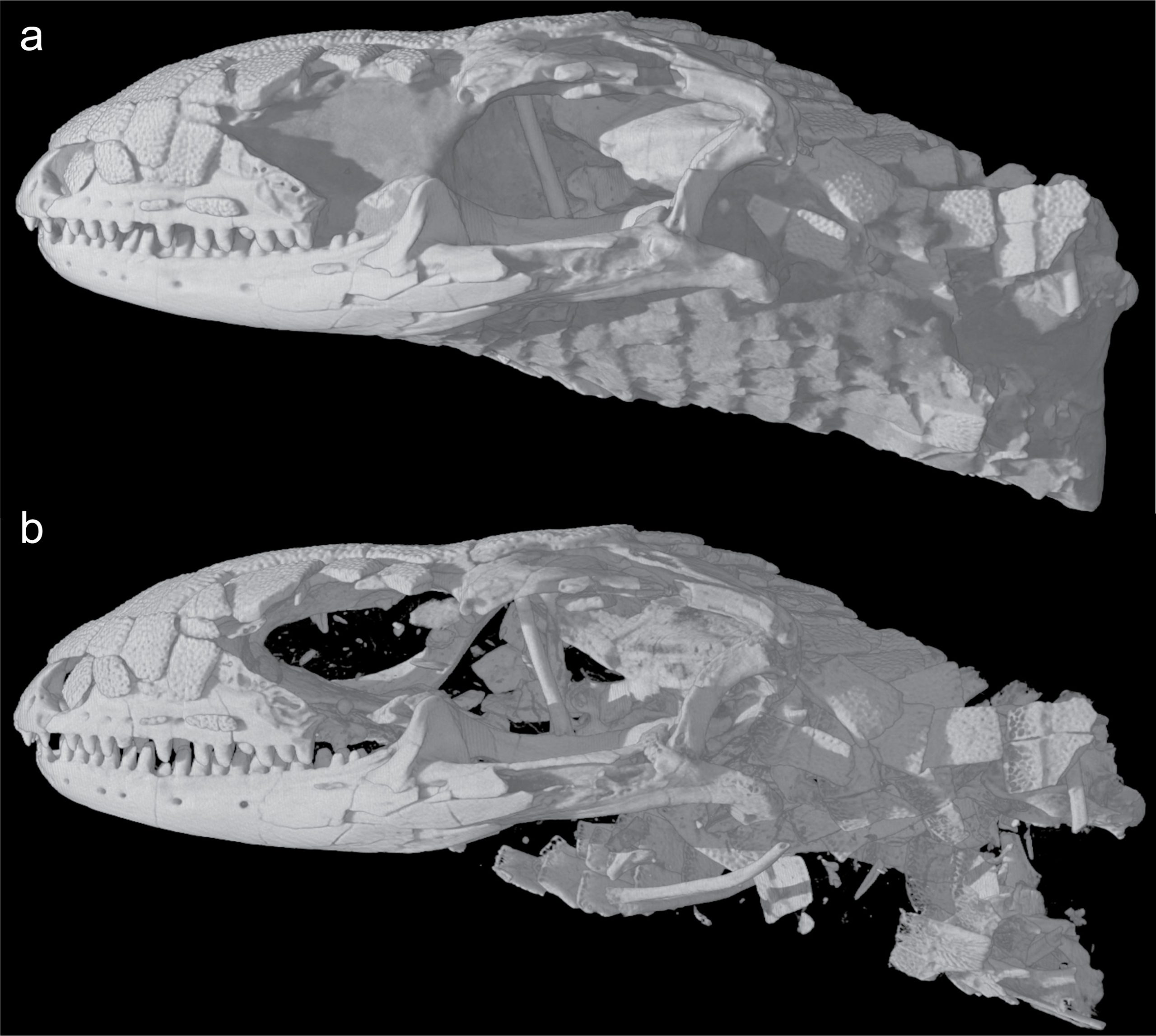
Recently, paleontologists have embraced the virtual world and computer-aided visualization to look at the three-dimensional structures in fossils. From this, they can better look at the fossil’s internal structure. Much like when your doctor needs to look at your organs in detail, paleontologists use computed tomography (CT) with multiple x-ray scans to look through a fossil.
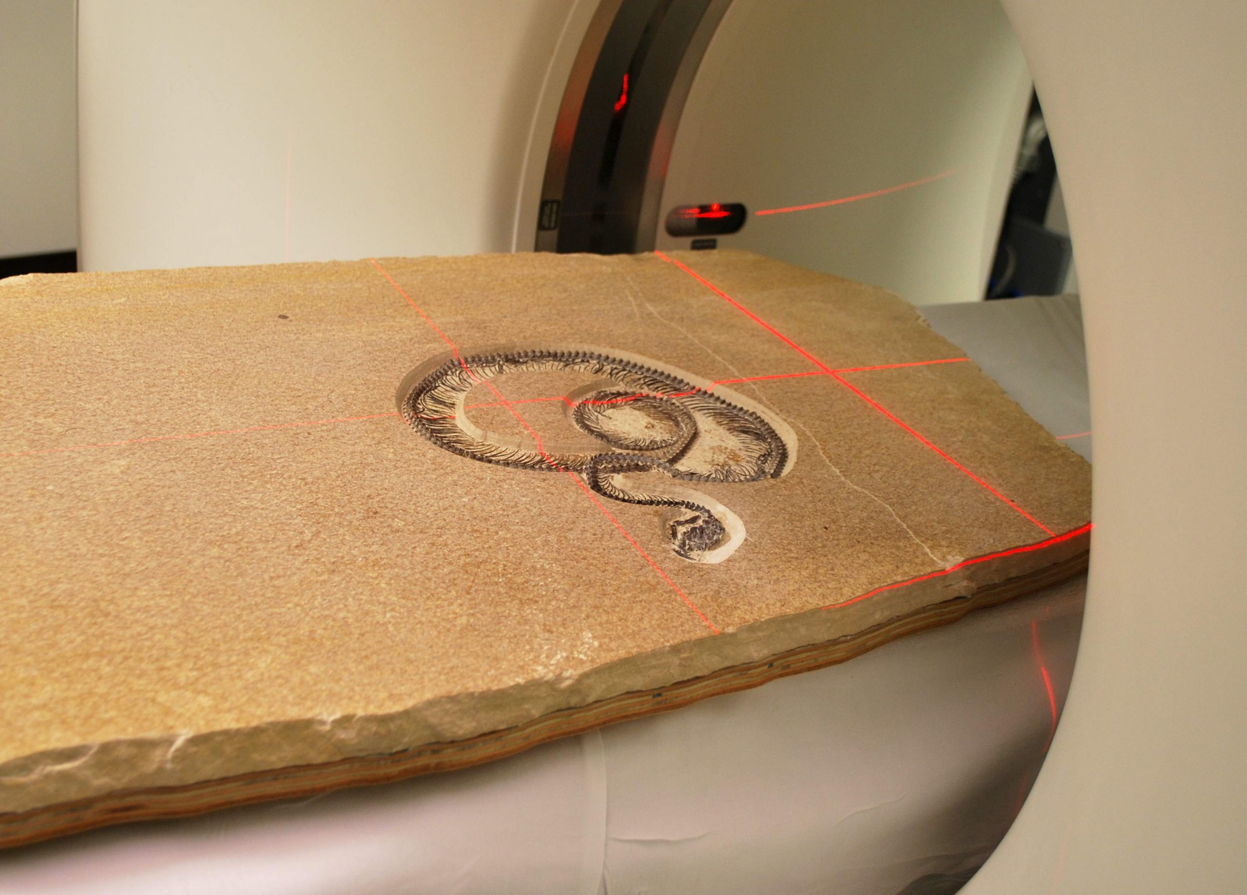
Using CT images also helps with fossil preparation as paleontologists often spend hours carefully removing rock matrix from a fossil. For example, if you have seen trilobite specimens, these are often prepared by micro air blasting with talc to remove the host limestone. This can take from a few to tens of thousands of hours. CT is much faster at digitally removing the rock matrix (Figure 7.2).
Even with newer techniques, the basics of looking at fossils have remained constant for centuries. In fact, some dismiss paleontology as a dead science because simple observations that are the backbone of paleontology are not seen as a credible test you do in a laboratory or model made with advanced machine learning. Paleontology is like a rosetta stone and can help you decipher the tapestry of Earth’s history and become a better scientist. If you remember the skills you have been using, such as sketching, data collection, and map interpretation, you’ll do well studying fossils.
7.2 Taxonomy
Taxonomy sounds like a big word, but it’s just the term used to describe how scientists classify things, which we’ve been doing throughout this lab manual (e.g. rock and minerals). The classification of fossils is one of the meeting points between geology and biology, and we follow the traditional biology taxonomy when classifying fossils (Figure 7.3). The major ranks are domain, kingdom, phylum, class, order, family, genus, and species. For the fossils in this lab manual, we will focus primarily on the phylum rank, with some organisms at the class and order rankings.
Exercise 7.1 – Taxonomic Rankings
Using your phones, laptops, or tablets, look up the taxonomic ranking of the species in Table 7.1.
| Ranking | Human | Bornean orangutan | Dog | Rice |
|---|---|---|---|---|
| Domain | ||||
| Kingdom | ||||
| Phylum | ||||
| Class | ||||
| Order | ||||
| Family | ||||
| Genus | ||||
| Species | sapiens | pygmaeus | lupus familiaris | sativa |
You can take an entire course dedicated to paleontology, so we will only cover the more common fossils in the following pages. These fossils have detailed anatomies that are used to differentiate class, order, family, genus, and species. In this chapter, we want you to be able to identify common fossils at a broad level. A detailed study is reserved for upper-level classes. Therefore, for most of these organisms, you will not see a detailed review of their anatomy.
Exercise 7.2 – Comparing Common Fossils
Your instructor will provide you with some common fossils. Create sketches of them and describe the differences that you can observe.
| Sketch of first fossil: | Sketch of second fossil: |
- What are the similarities and differences between these fossils?
- Critical Thinking: What evidence from these fossils suggests that they may be organisms that are now extinct?
- How would you respond to someone who argues that all fossils that are thought to be extinct are actually still alive but haven’t been “rediscovered” yet?
The geologic record is full of fossils, from dinosaurs to plants to fish and everything in between. Invertebrate animals from the marine environment are the most common branch of fossils you will find because of their abundance and higher probability of fossilization versus land-dwelling organisms, and they will be the focus of this chapter. Table 7.2 contains a list of the major marine invertebrate phyla we will cover, and in some cases, the class and order.
| Phylum | Class | Order | Common Names |
| Cnidaria | Anthozoa | Rugosa, Tabulata, Scleractinia | Rugose (horn) coral, tabulate coral, scleractinian coral (stony or hard coral) |
| Bryozoa | Bryozoan | ||
| Mollusca | Bivalvia, Cephalopoda, Gastropoda | Clam, squid, snail | |
| Brachiopoda | Brachiopod | ||
| Arthropoda | Trilobita | Trilobite | |
| Echinodermata | Echinoidea, Crinoidea, Blastoidea, | Sand dollar, crinoid, blastoid, starfish |
7.3 Symmetry
A helpful characteristic in identifying fossils is the symmetry of the organism. Symmetry is an observable pattern in the external or internal structure of organisms that allows you to divide that organism into roughly equal parts that are mirror images of each other. For example, take the face of a human being which has a plane of symmetry down its center, an example of external symmetry. Internal features can also show symmetry. For example, the tubes in the human body, such as your arteries and veins, are cylindrical and have several planes of symmetry. Most multicellular organisms have some form of symmetry.
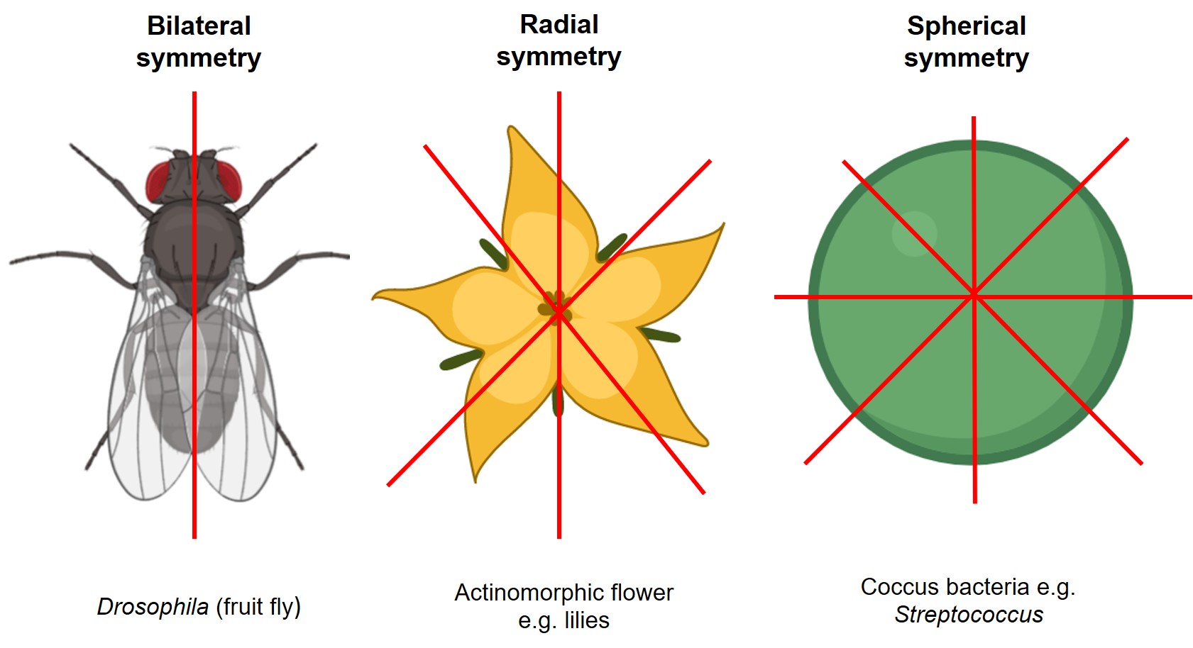
There are several types of symmetry in biology, but the main ones you will see are bilateral, radial, and spherical (Figure 7.4). Bilateral symmetry is a single plane that divides the organism into two equal, mirror-image halves. Radial symmetry has several subtypes, but they all describe symmetry lines drawn through a central point. The common types of radial symmetry for fossils in this chapter are 5-fold radial symmetry (pentamerous) and 6-fold radial symmetry (hexamerous). Spherical symmetry is when you can draw a line of symmetry through a central point of the organism from any direction so that no matter what the orientation of your symmetry line is, you will always have two equal, mirror-image halves.
Exercise 7.3 – Identifying Symmetry in Fossils
Let’s get some practice identifying and describing the differences in symmetry.
- Your instructor will provide you with a selection of fossils that exhibit bilateral, radial, spherical, or no symmetry. On a separate sheet of paper, create a sketch of each fossil that highlights its symmetry. Be sure to draw the line(s) of symmetry on your sketch and indicate which type of symmetry each fossil has.
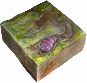
- Critical Thinking: Recently, Evans et al. (2020) described Ediacaran fossils of Ikaria wariootia (Figure 7.5) found in South Australia as the first organisms with bilateral symmetry. Ikaria have also been linked to a Nereites-type trace fossil. What would be the benefit of this type of symmetry for these organisms?
7.4 Phylum Cnidaria
Cnidaria is a phylum of marine organisms that includes over 11,000 species, including jellyfish, sea anemones, and coral; most have radial symmetry. The soft bodies of jellyfish and sea anemones are rarely preserved, whereas the hard structures of corals are quite commonly preserved as fossils. In the geologic record, three orders of coral are the most abundant: rugose, tabulate, and scleractinian corals. Corals are carnivores, catching zooplankton with their tentacles and pulling them into their mouths. Some corals also have a partnership with green algae that live within the coral. As the algae perform photosynthesis, some of the energy they create is transferred to the coral.
Order Rugosa
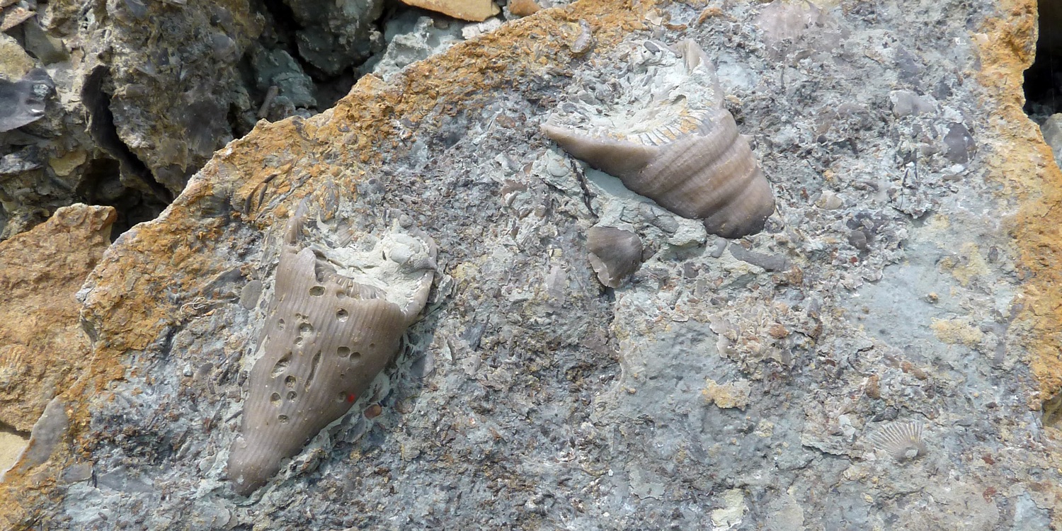
Rugose corals (Figure 7.6) are an extinct order of coral that originated in the Ordovician and went extinct at the end of the Permian. Members of Rugosa are sometimes called horn corals because solitary forms frequently have the shape of a bull’s horn (if you like the Harry Potter movies, some say they look like the sorting hat). Rugose corals do have a less common, colonial form that does not have this shape.
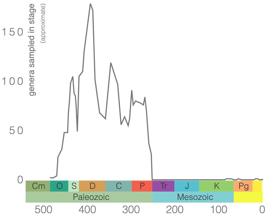
Rugose corals reached their peak diversity during the Devonian period when colonial forms were important reef builders (Figure 7.7). They went extinct during the end-Permian mass extinction event. Figure 7.7 is the first of many diversity curves you will see in this chapter. Diversity curves allow paleontologists to graph how many different kinds of fossils existed on earth during different geological time intervals. They are especially important for telling us (a) when a group of animals first evolved on earth, (b) when that group diversified (increased in diversity) and became common on earth, and (c) when that group went extinct.
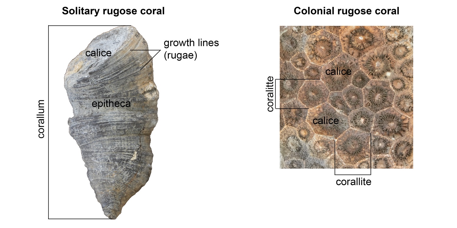
Rugose corals may be either solitary or colonial (Figure 7.8). A solitary coral individual is called a corallum, while an individual within a colony is called a corallite. Rugose corals made their skeletons from calcite; this is a significant difference relative to other corals that make their skeletons out of aragonite, which is more resistant to stress.
The outer part of the corallum (or corallite) is called the theca; think of it as the skeletal wall (Figure 7.8). The theca may, in turn, be covered by an outermost skeletal sheath called the epitheca. Growth lines are often apparent on the epitheca; these are also called rugae (“ruga” is Latin for wrinkled), which gives this group of corals their scientific name (thus, rugose corals are the “wrinkled corals”). Finally, the top of the corallum (or corallite) is called the calice, and it is the portion of the coral occupied by the living organism, called a polyp.
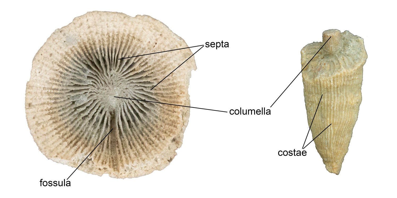
The surface of the calice is covered with radiating, vertical structures called septa (singular = septum) that resemble the spokes of a bicycle wheel (Figure 7.9). Septa sometimes extend through the theca, forming vertical lines called costae (singular = costa). The septa radiate outwards from a central pillar-like structure called the columella. In rugose corals, the septa are added during growth in a manner that ultimately divides them into four quadrants. Spaces between the four quadrants are called fossula. However, it is important to note that fossula are not readily visible in many specimens, especially when they are poorly preserved.
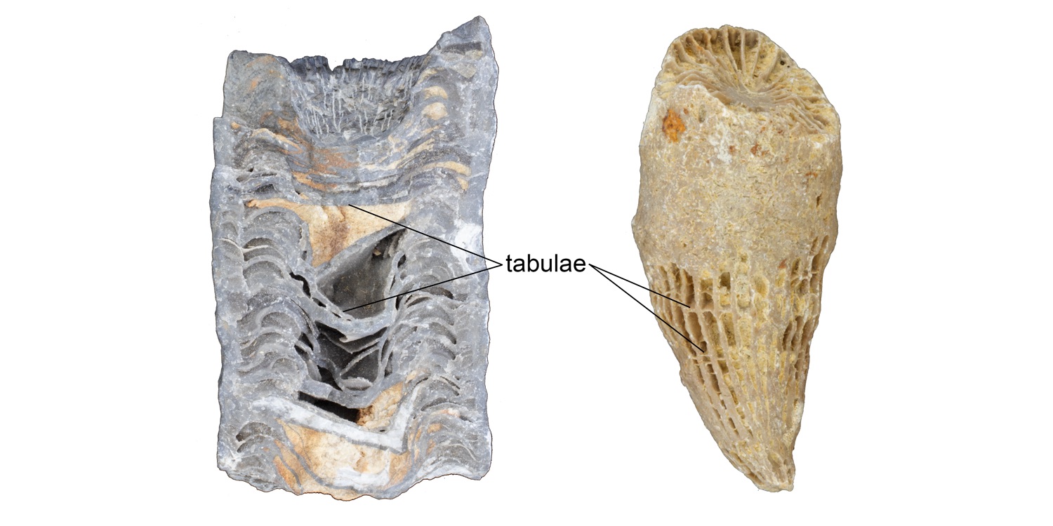
As a coral polyp grows upwards, it develops horizontal partitions called tabulae (Figure 7.10).
3-D Model 7.1 – Rugose Coral
This is a model of the rugose coral Heliophyllum halli from the Middle Devonian from Moscow. The growth lines and costae are clearly visible on the epitheca. Some septa are the only visible features on the calice.
More 3-D models of rugose corals can be found at the Digital Atlas of Ancient Life.
Order Tabulata
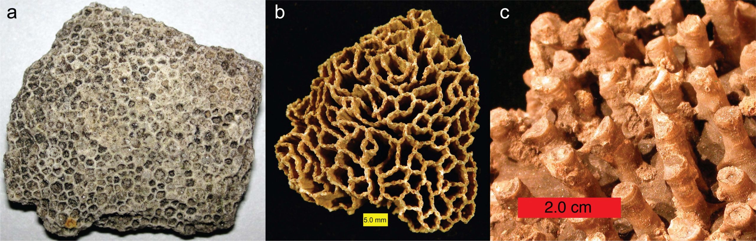
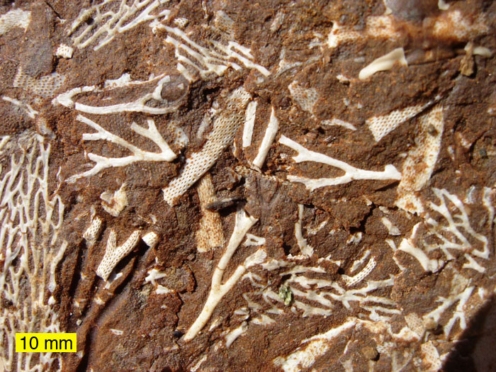
Tabulate corals originated in the Early Ordovician period and went extinct at the end of the Permian period. All tabulate corals were colonial, and some species were important reef makers during the Silurian and Devonian periods. Tabulate corals constructed their skeletons primarily of calcite. Some tabulate corals look superficially like honeycombs (e.g., Favosites; Figure 7.11a), while others look like chain links (e.g., Halysites; Figure 7.11b) or collections of narrow tubes (e.g., Syringopora; Figure 7.11c). Others can be encrusted upon other marine invertebrates (including other corals).
The following video from the Paleontological Research Institute gives a great introduction to tabulate corals.
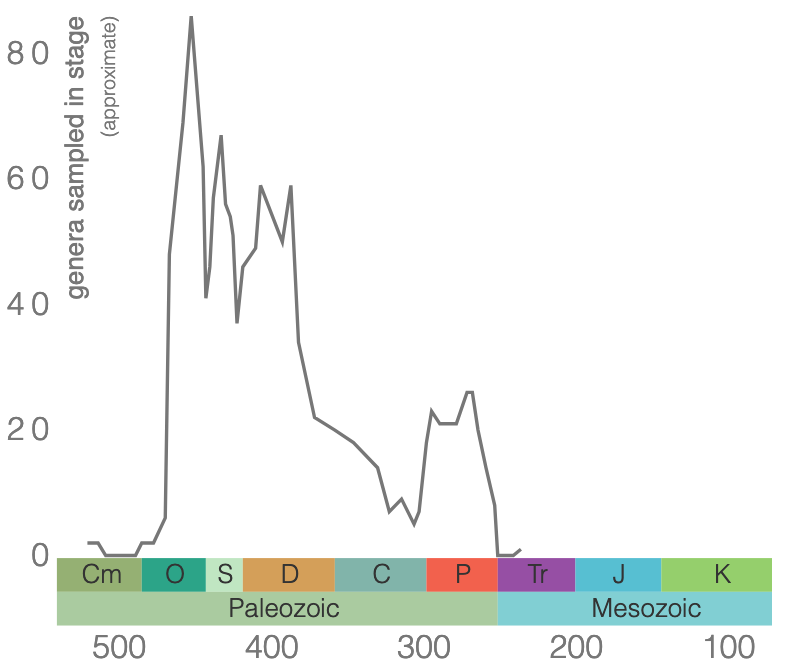
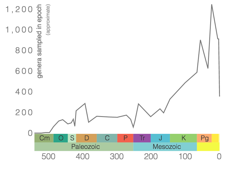
According to the Paleobiology Database, there are 58 families of tabulate corals, 376 genera, and 511 species. As demonstrated by the genus-level plot of their diversity through time (Figure 7.12), tabulate corals suffered badly during the Late Devonian extinction event and never again reclaimed their former levels of diversity. The group went extinct at the end of the Permian period.
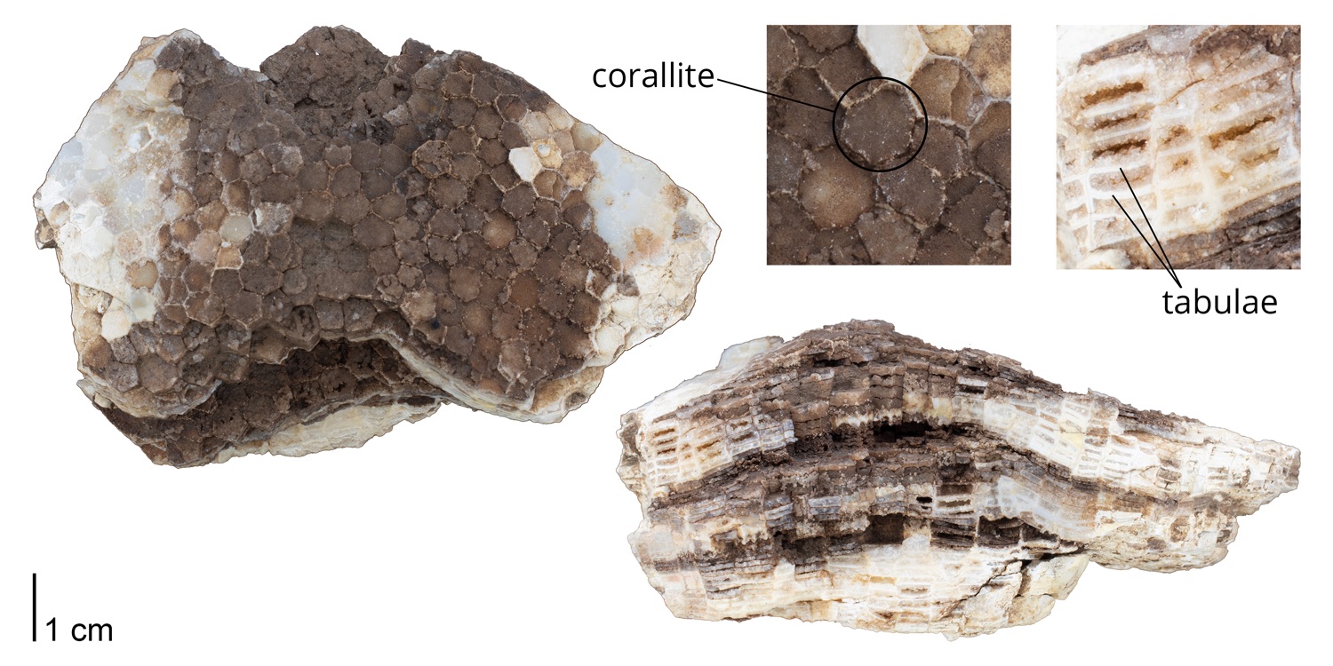
A defining feature of most tabulate corals are structures called tabulae, which give them their name. Tabulae (singular, tabula; from the Latin for board or tablet) are horizontal plates that span across individual corallites (Figure 7.13). They are deposited by polyps as they grow, separating the living animal from the space(s) occupied earlier in life. Remarkably, we know something about the soft polyps of tabulate corals due to the discovery of calcified polyps in specimens of Silurian Favosites from the Jupiter Formation of Quebec, Canada. This discovery was reported by Copper (1985), who reported that individual corallites typically had 12 tentacles, though some had 11 or 13. The discovery of these polyps also confirmed that Tabulata are indeed Cnidarians, rejecting the hypothesis of some earlier workers that this group belonged with the sponges.
Unlike rugose and scleractinian corals, most tabulate corals did not have septa. Therefore, as a general rule, identifying whether or not a specimen of colonial Paleozoic coral has septa is a good indication of whether it is a rugose coral (septa always present) or a tabulate coral (septa usually absent).
3-D Model 7.2 – Tabulate Corals
This is a model of the tabulate coral Favosites favosus from the Silurian of Delaware County, Iowa (PRI 76737). It is the same one pictured in Figure 7.12. The length of the specimen is approximately 10 cm. The specimen is from the collections of the Paleontological Research Institution, Ithaca, New York. The side view shows the tabulae, and the top view shows the corallites.
Order Scleractinia
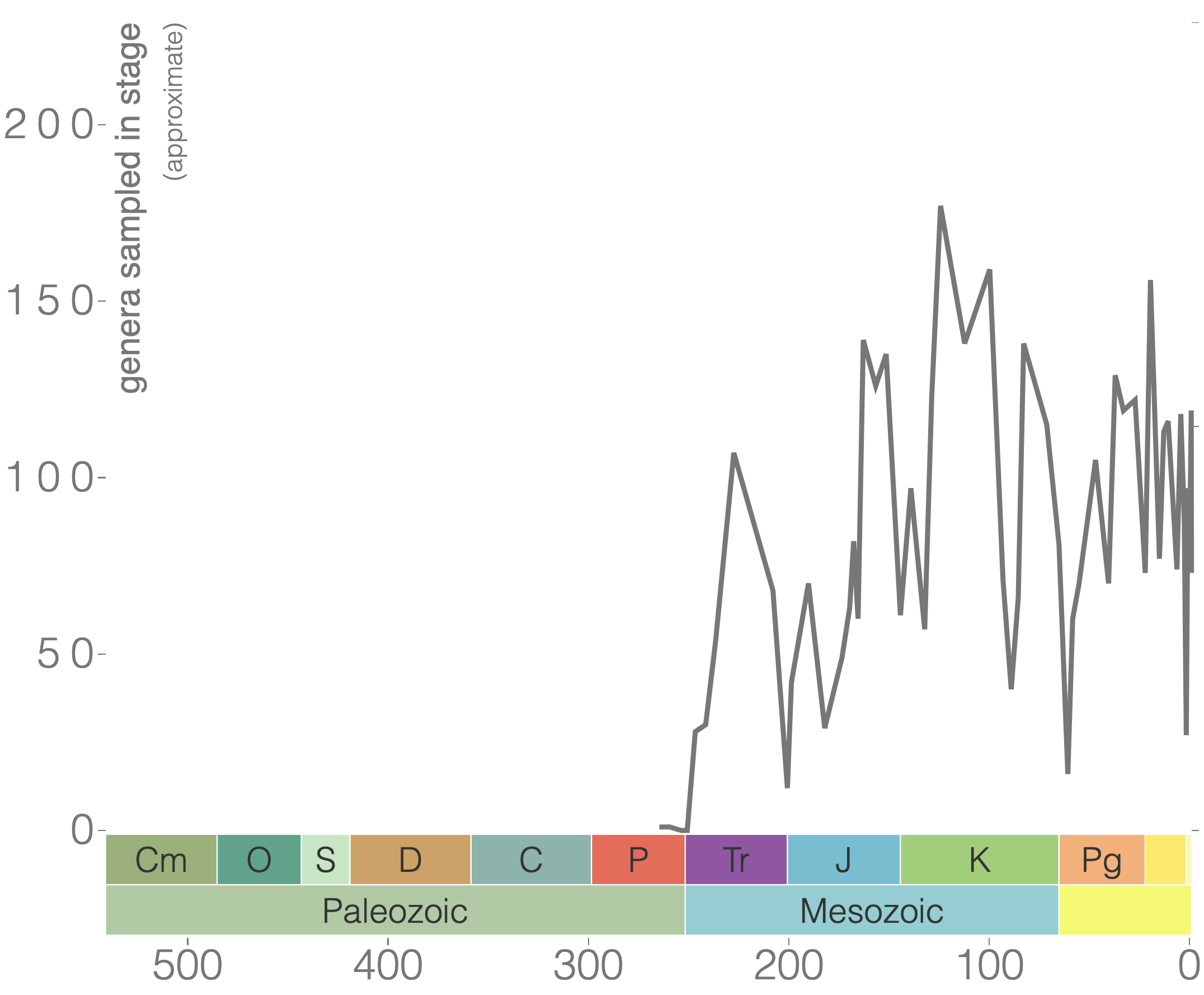
The order Scleractinia includes the “true corals” or “stony corals,” with about 1,500 living species today. Scleractinians first appeared in the early Middle Triassic (Figure 7.14) and have been the dominant reef-building organisms over the past 240 million years.
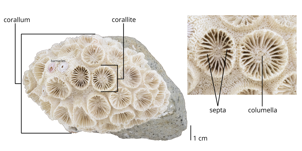
Scleractinian corals may be either solitary or colonial in form and always have skeletons composed of aragonite. We are going to focus on the colonial forms of Scleractinia corals. An entire colonial coral colony is a corallum; the space occupied by a single polyp within the colony is called a corallite (Figure 7.15). Individual corallites have their own radial septa, which often attach to a centralized pillar called the columella; all familiar terms from rugose and tabulate corals.
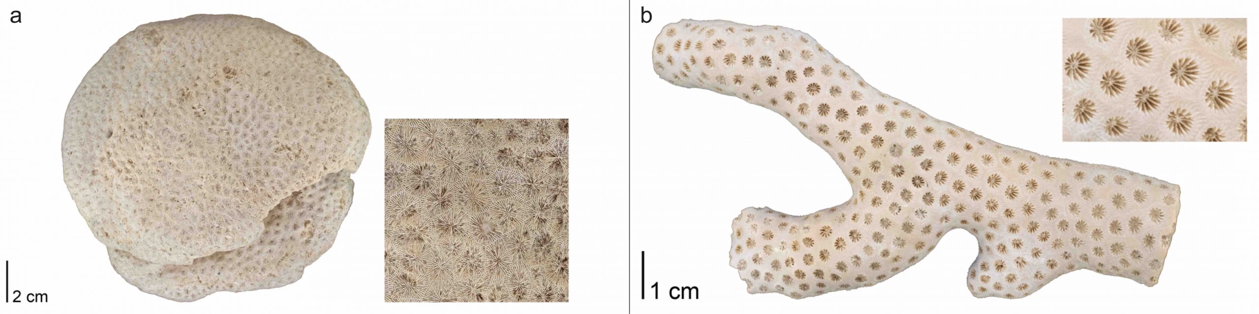
The skeletons of colonial corals exhibit a much greater diversity of forms than those of solitary species. Often, their growth forms are dependent upon the habitats in which they live. For example, robust, rounded colonies are often favored in high-energy habitats with lots of wave action (Figure 7.16a), while delicate branching forms are usually associated with quieter environments (Figure 7.16b).
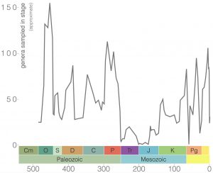
7.5 Phylum Bryozoa
Bryozoans are filter-feeding invertebrates found in freshwater and marine habitats, where they are often easy to miss because of their small size (Figure 7.17). In almost all species, tiny (<1 mm diameter) bryozoan individuals, called zooids, live together as a colony that often encrusts surfaces, grows branching structures, or, in freshwater species, forms a gelatinous blob. They have bilateral symmetry. Despite their small size, marine bryozoans are abundant in many fossil assemblages thanks to the preservation of their hard calcium carbonate skeletons. Bryozoans first appeared in the Ordovician and are still present in oceans today (Figure 7.18). They were greatly impacted by several mass extinctions with their lowest diversity occurring during the Mesozoic. More than 17,800 species of fossil bryozoans have been described, and more than 6,000 living species are known.
Bryozoan colonies have highly variable forms (Figure 7.19), from gelatinous blobs to upright branching structures and sheet-like encrusters, but the general morphology of a zooid is similar across the classes. Zooids can take several forms, but the most common forms in each class are autozooids, which function in feeding the colony and excreting waste. Branching bryozoans may look similar to branching corals, but the zooids in bryozoa do not have septa or a columella as corallites do in corals.
7.6 Phylum Mollusca
Mollusks are a phylum of marine invertebrates that comprise about 23% of all marine organisms. There are several classes of mollusks, but we will focus on gastropods, cephalopods, and bivalves. All have bilateral symmetry, but it’s more complicated for gastropods.
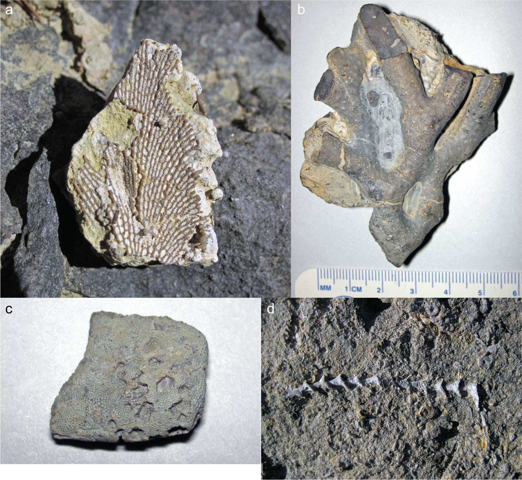
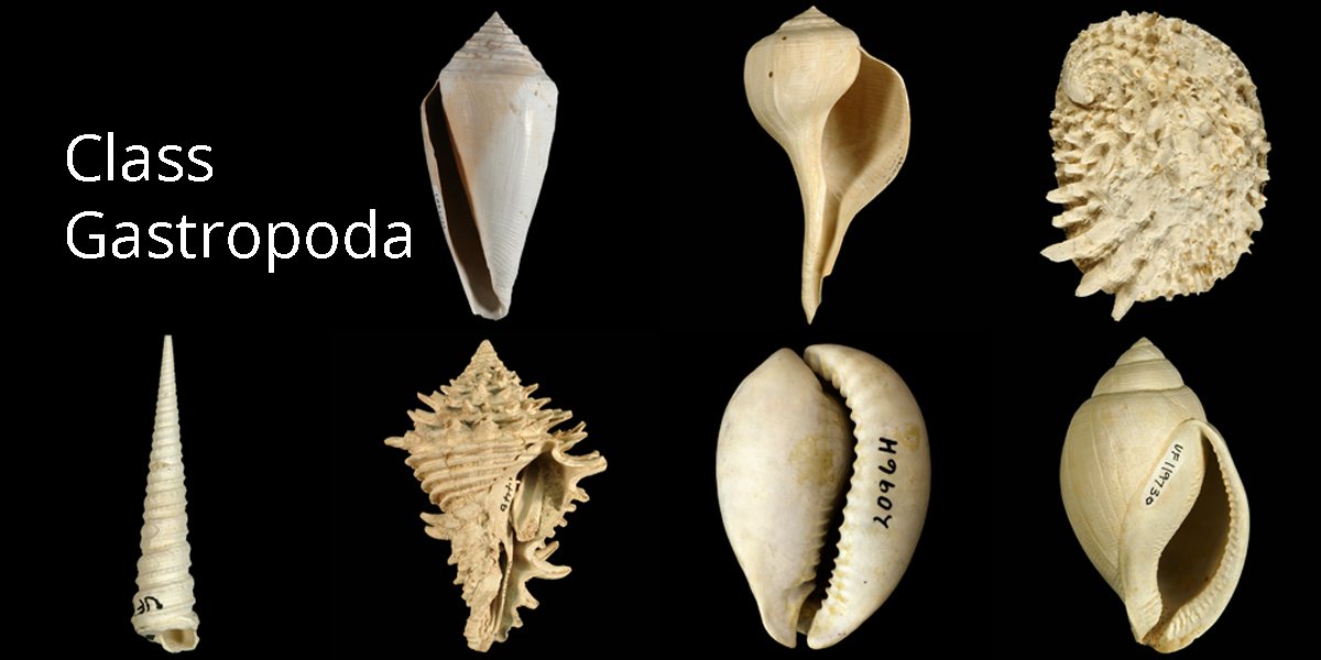
Class Gastropoda
Gastropods are one of the most evolutionarily successful groups of animals; you may commonly know them as snails and slugs. They occupy the world’s oceans, freshwater lakes and streams, and terrestrial ecosystems, including many backyards. Some are algae-eating herbivores, while others are venomous hunters of fish. Their strong, single-valved shells (Figure 7.20) have left behind a rich Cambrian to Recent fossil record and are the focus of many paleobiological studies (Figure 7.21). These shells are primarily made of calcium carbonate. Gastropods have many different shell shapes, and some with no shell, but one of the defining characteristics of gastropods is the rotation of their body during their development, a process called torsion. Torsion does not refer to the coiling shells you are familiar with and only relates to the gastropod’s coiled body. Before rotation, gastropods exhibit bilateral symmetry, but they lose that symmetry as they mature.
Class Cephalopoda
Cephalopods are marine organisms with bilateral body symmetry, a prominent head, and a set of tentacles. You may be familiar with some of them, like squids and octopuses. While most modern cephalopods are completely soft-bodied or have only thin internal shells, their ancient shelled cousins left behind a detailed fossil record with a remarkable diversity of shell shapes. Cephalopods became abundant during the Ordovician Period, and many went extinct by the end of the Mesozoic Era with the dinosaurs (Figure 7.22).
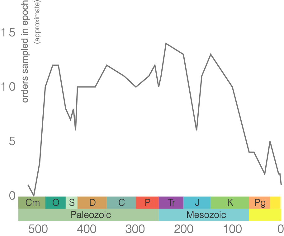
One of the most well-known index fossils for cephalopods is the belemnite (Figure 7.23). The belemnite is an extinct order of mollusk that only lived during the Mesozoic. It had a characteristic elongated, cone-shaped shell called a guard (Figure 7.23b). The guard is thought to have been a counterbalance that allowed the belemnite to move horizontally through the water.
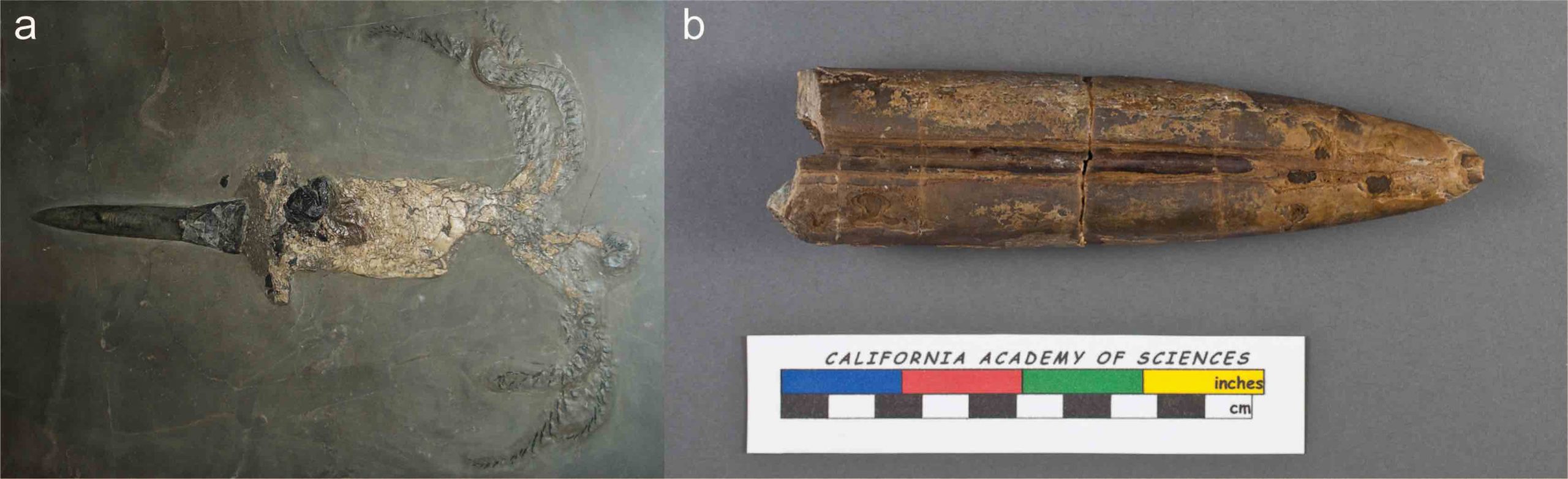
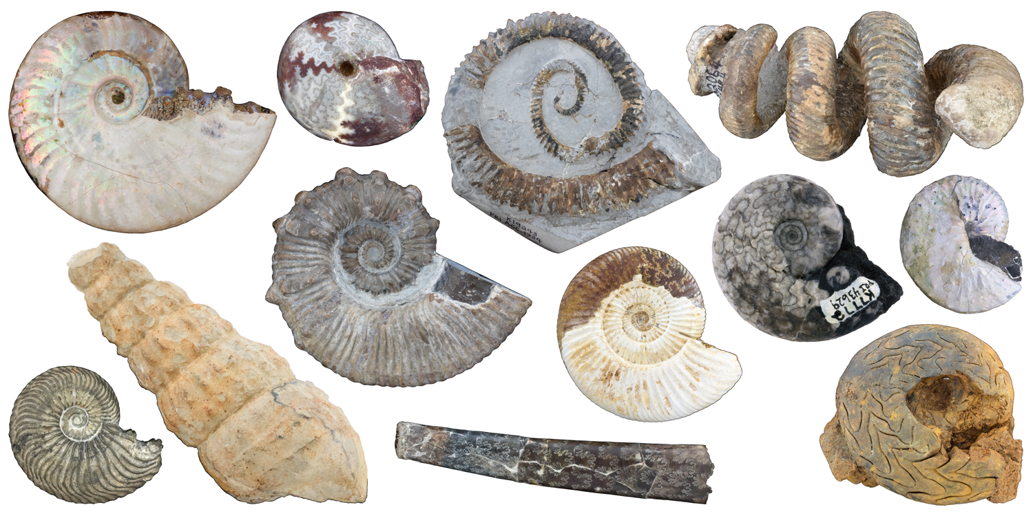
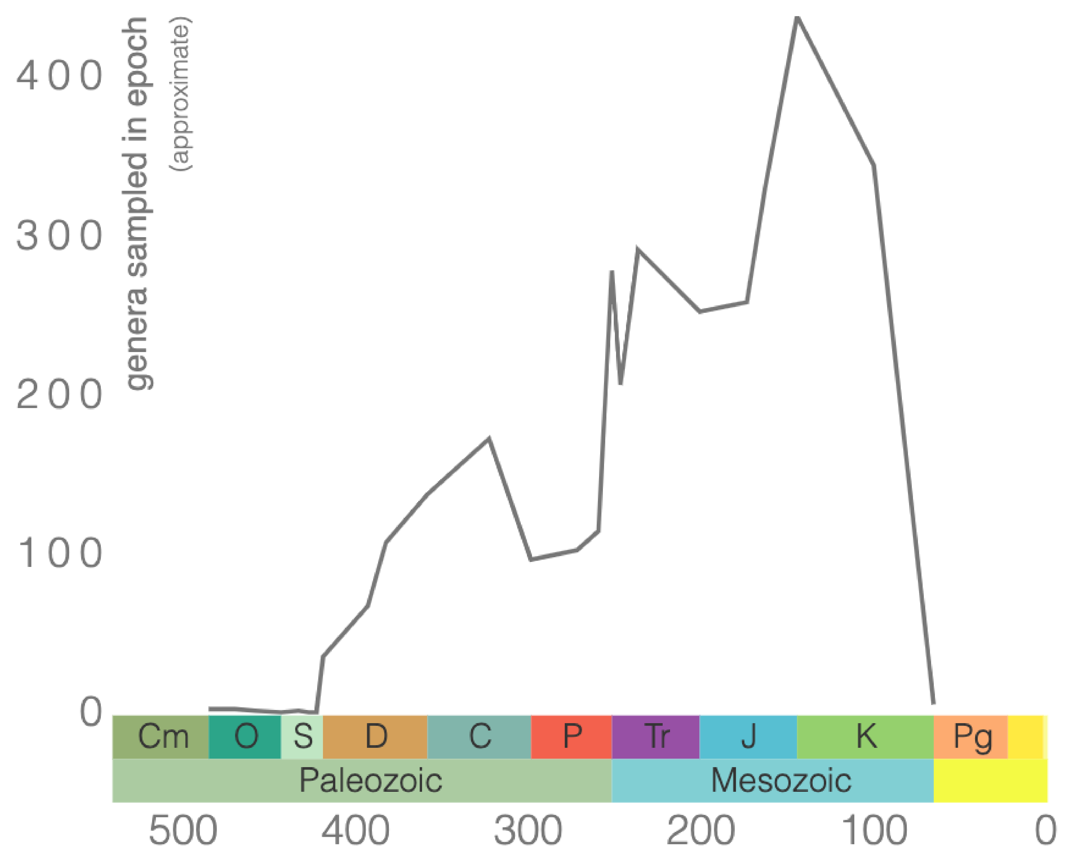
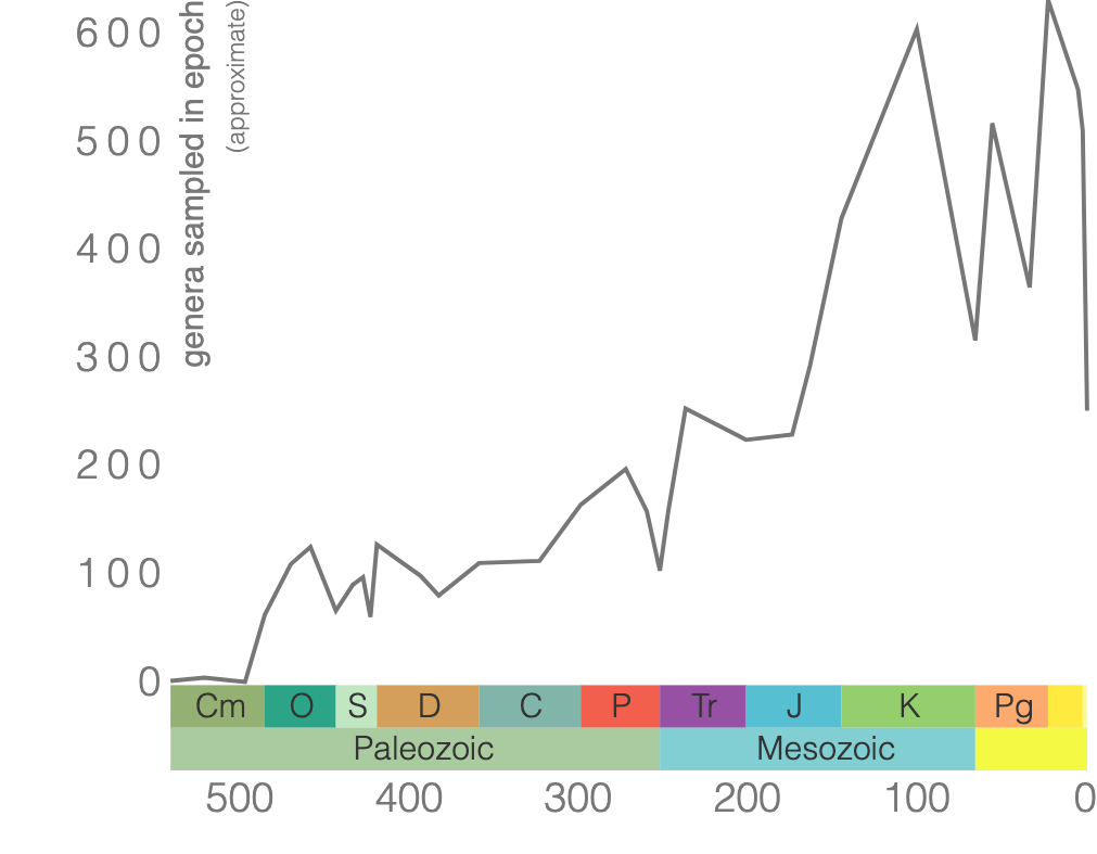
Other well-known cephalopod index fossils are from the subclass Ammonoidea, commonly referred to as ammonites (Figure 7.24). They are extinct mollusks that lived from the Devonian to the end of the Cretaceous (Figure 7.25). These are ideal for biostratigraphy as there are over 8,000 species of ammonoids, and they occur over a large geographic range.
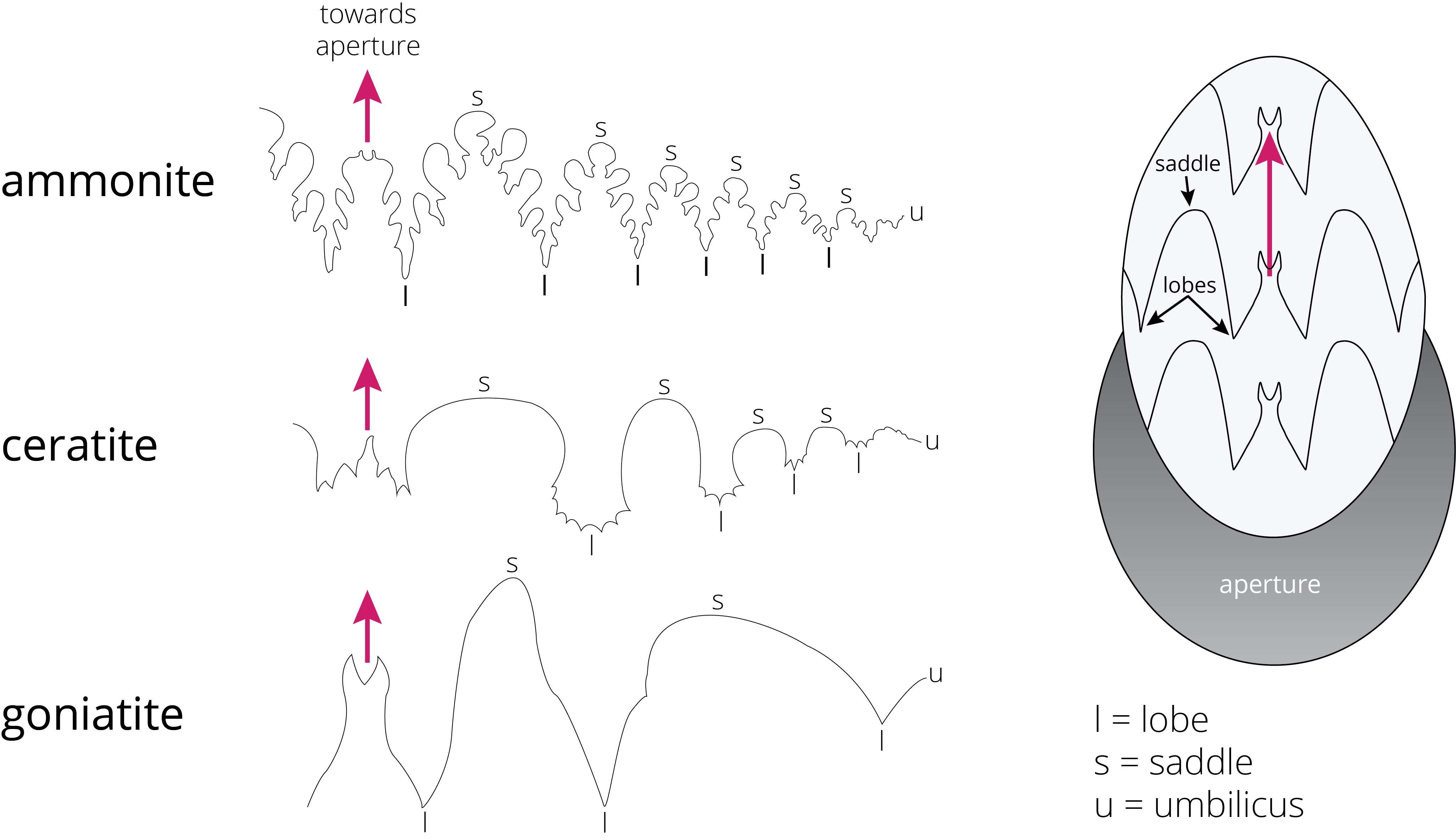
One of the ways to distinguish orders of ammonoids is the suture pattern of their shells (Figure 7.26). Ammonoid sutures fall into three main groups: goniatites, ceratites, and ammonites. As you go from goniatites to ceratites to ammonites, the suture patterns become more complex. Goniatitic sutures do not have subdivided saddles or lobes. Saddles are convex toward the opening of the shell, and lobes are convex in the other direction. Ceratitic sutures have subdivided lobes but undivided saddles. Finally, both the saddles and lobes of ammonitic sutures are subdivided, sometimes in an amazingly complex fashion.
One of the oft-quoted principles of evolutionary theory is, “ontogeny recapitulates phylogeny.” This a historical hypothesis from Ernst Haeckel that states the development of the embryo of an animal, from fertilization to gestation or hatching (ontogeny), goes through stages resembling or representing successive adult stages (recapitulates) in the evolution (phylogeny) of the animal’s remote ancestors. It means that as an animal develops, different stages of growth may give you hints of the evolution that their ancestors went through. Modern biology is full of examples of this theory.
Well, for the fossil record, this theory is hard to prove because of incomplete preservation. One of the best examples in the fossil record that supports this quote is the suture patterns in ammonite shells. These sutures form at the intersection of the shell wall and the interior septa (walls dividing the interior cavity). These patterns started as mere wavy lines in the Cambrian and became more complex through time. Through time, the sutures acquired additional saddles and lobes. Later, paleontologists recognized that within some species, such as a Permian ammonoid (Perrinites), the sutures are simple patterns in young animals and get more complex as the animal gets older. Thus, the suture patterns in the young animals resemble their ancestors.
Exercise 7.4 – Stratigraphic Analysis and Fossil Evolution
On a class field trip to the Guadalupe Mountains in west Texas (Exercise 6.4), you are taken to a stratigraphic section that goes through the Carboniferous to Permian up to the Capitanian extinction, which was an extinction event that occurred in the late Permian about 260 Ma. Your field trip leader has given you a guide to some of the important ammonite species used for relative age dating in this area. In addition, she has given you the patterns for several ammonite species. You prefer looking at fossils compared to stratigraphic sections and have found two fossils just randomly on the ground. Can you place these on the stratigraphic column?
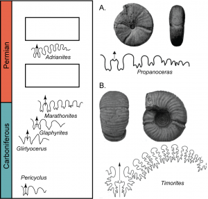
- Describe how the sutures of species in this stratigraphic column evolve through time.
- Based on the evolution of the suture patterns, place these two unknown fossils in the column. You can sketch the sutures in the blank boxes.
- Explain your answer.
Class Bivalvia
Bivalves refer to a diverse Mollusca class that typically has bilateral symmetry where the upper shell and inner parts of the organism are a mirror image of the bottom half. Clams, oysters, and mussels belong to this class. Their shells are made of calcium carbonate and typically have growth lines (Figure 7.28). Bivalves first appeared in the fossil record in the Cambrian and are still around today (Figure 7.29).
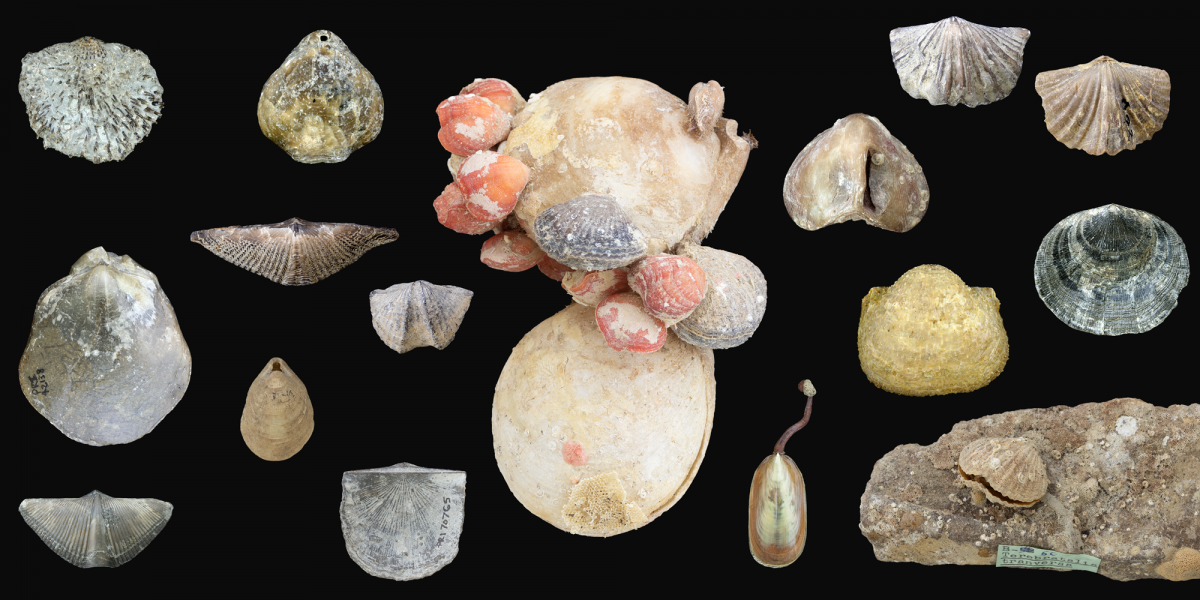
7.7 Phylum Brachiopoda
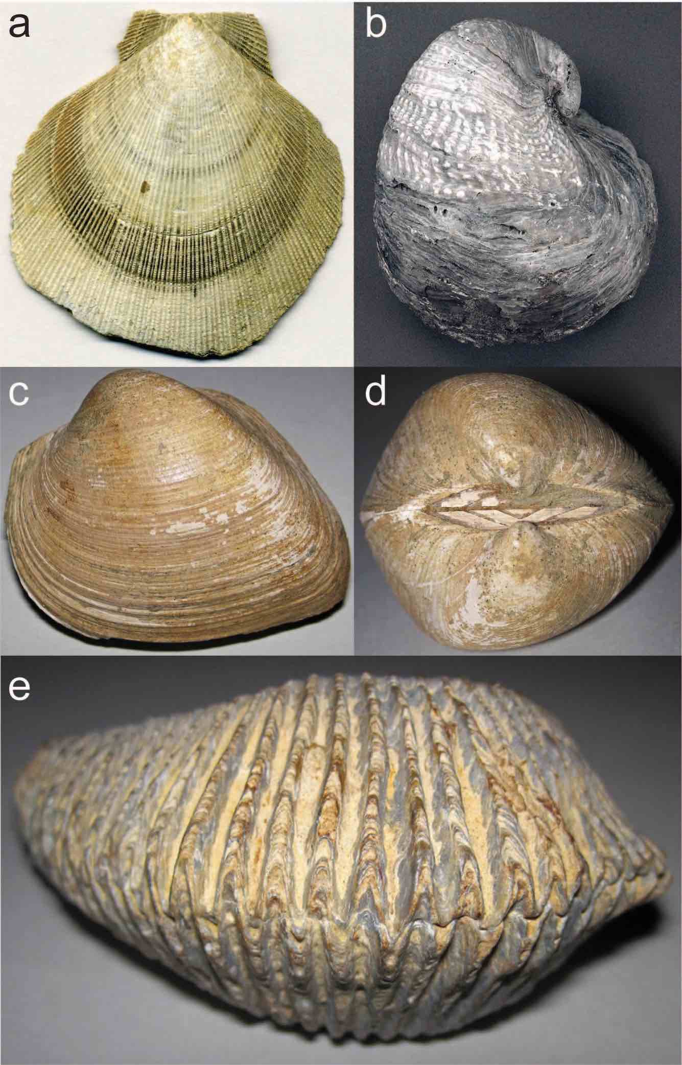
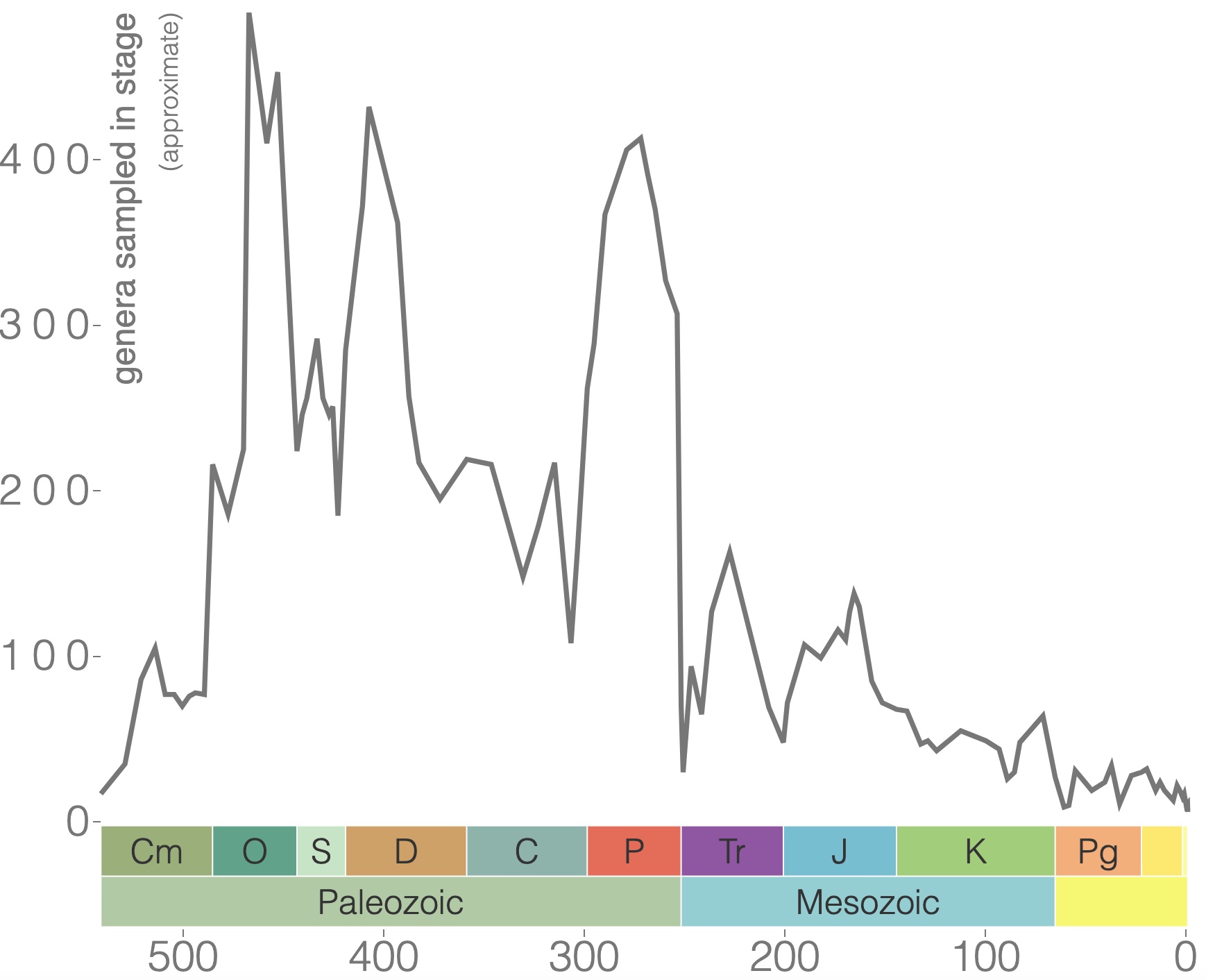
Brachiopods are shelled, filter-feeding marine organisms (Figure 7.30) that inhabit the seafloor and come in various shapes and sizes. They have been around since the Cambrian with incredible diversity during the Paleozoic Era (Figure 7.31). Brachiopods are still around today, but their diversity is greatly diminished.
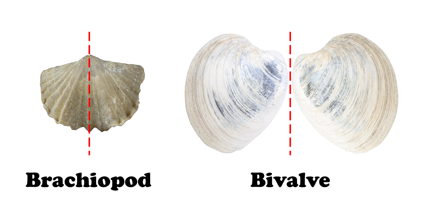
Superficially, brachiopods may look like bivalves, but the two are not related. One of the biggest differences between brachiopods and bivalves lies in their symmetry. Both have bilateral symmetry, but the plane of symmetry in brachiopods is vertical rather than horizontal (Figure 7.32). This means that the left half of a brachiopod is a mirror image to the right half. In bivalves, the plane of symmetry is horizontal, and the upper half is a mirror image of the lower half.
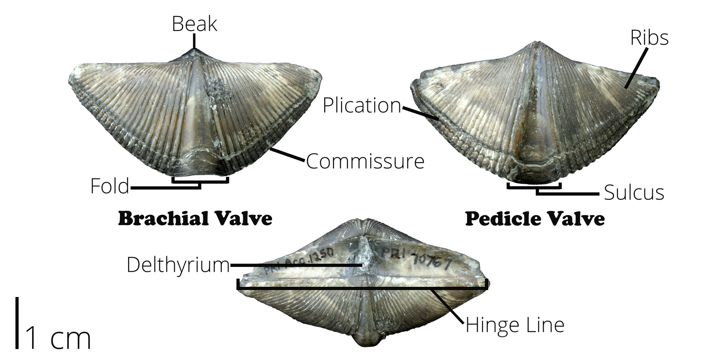
Brachiopod shells have two valves that are distinct in both size and shape (Figure 7.33). The brachial valve is usually the smaller of the two valves and has a ridge, or fold, down the middle of the valve. The pedicle valve is usually larger than the brachial valve and has a valley down the middle. It also has a hole through which the pedicle passes. The pedicle is a fleshy, stalk-like feature which some groups use to attach themselves to hard rocky seafloor. It is rarely preserved, but brachiopod shells will often have a pedicle opening preserved along the hinge-line that varies in shape from rounded to triangular.
7.8 Phylum Arthropoda
Arthropods are an extremely diverse and abundant phylum of animals. They include organisms such as spiders, scorpions, crabs, barnacles, and insects. Unfortunately, most of these are not abundant in the fossil record because of poor preservation, but one class of arthropods does stand out in the fossil record, the trilobite.
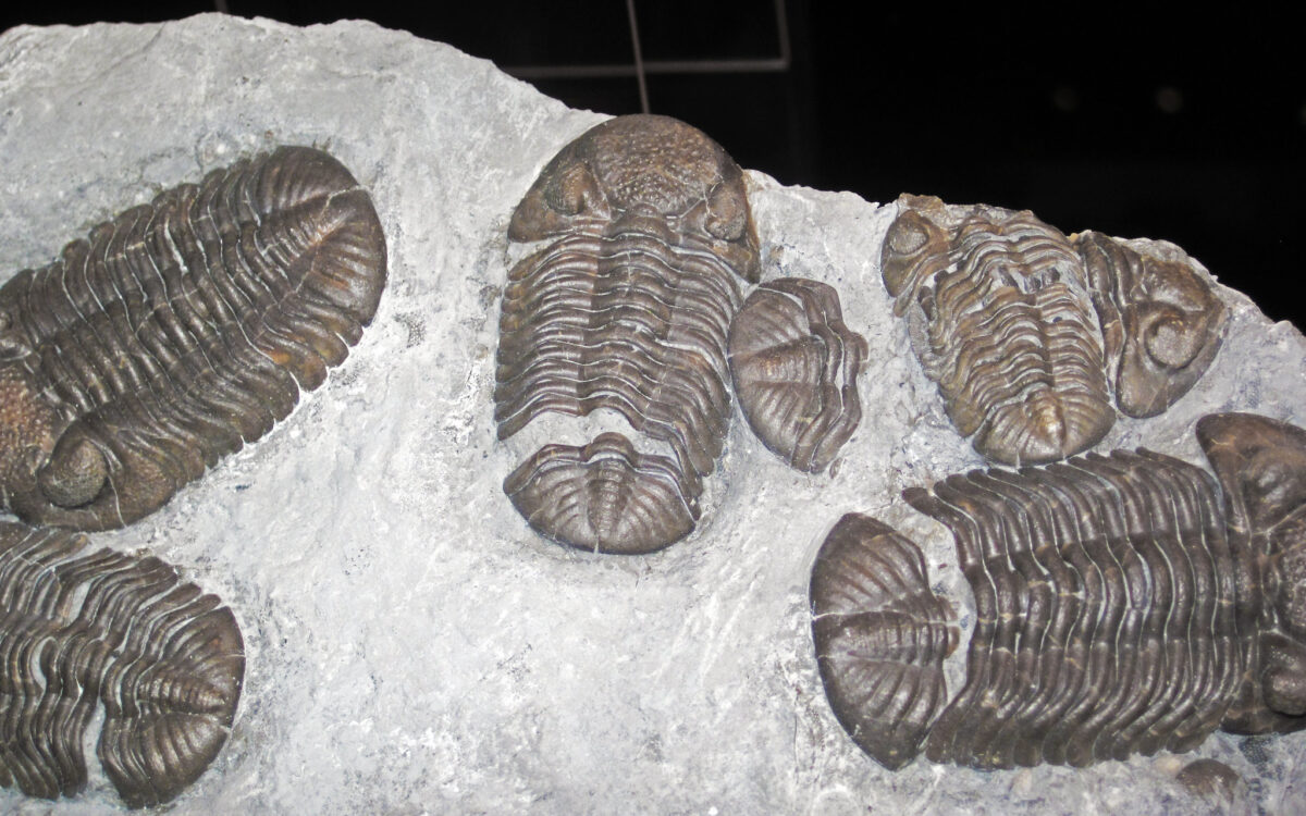
Class Trilobita
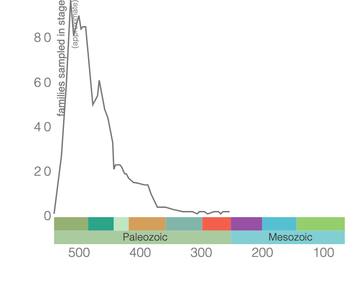
Trilobites are among the most well-known fossils, thanks largely to their abundance, diversity, and broad distribution during the Paleozoic (Figure 7.34). These emblematic arthropods first appeared in the fossil record 521 million years ago and survived until the end-Permian extinction approximately 250 million years ago (Figure 7.35). Even when they first appeared, trilobites were diverse and widespread, suggesting a long history before the first fossils, likely extending as far back as 700 Ma. During the Cambrian, trilobites were a dominant marine ecosystem component, but many of the Cambrian trilobite species died out during the extinction at the end of the Ordovician. Though the class did survive this extinction, their diversity never matched their earlier history. Because they evolved rapidly and were relatively widespread, trilobite species are often used to provide relative ages of the rocks in which they are found.
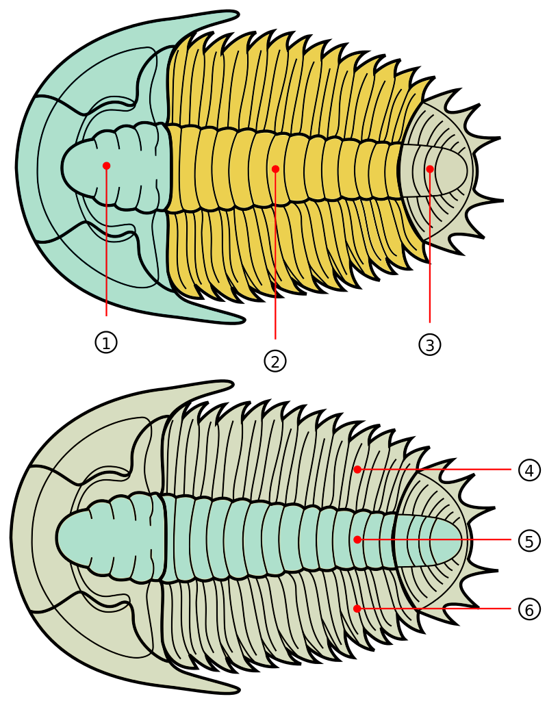
Trilobites get their name because their bodies exhibit three distinct, longitudinal sections, and they also have three segments from “head to toe” (Figure 7.36) and have bilateral symmetry. They fed in several ways, including moving across the ocean floor as predators, scavengers, or filter feeders, and some swam to feed on plankton. They ranged in size up to 45 centimeters long (about 1.5 feet).
7.9 Phylum Echinodermata
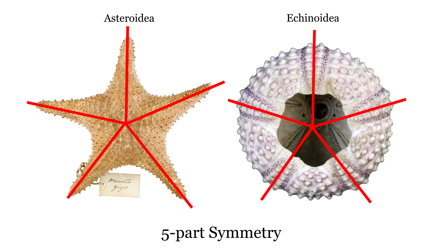
Echinoderms represent the largest marine animal phylum and include starfish, sea cucumbers, sand dollars, blastoids, and crinoids. They first appeared in the fossil record in the Cambrian and are still around today. One of the key features of this group is five-part, radial symmetry (Figure 7.37). There are many classes of echinoderms, and we will focus on Echinoidea, Crinoidea, and Blastoidea.
Class Echinoidea
Echinoids are the most diverse echinoderm class (Figure 7.38). They include spiny-looking sea urchins (regular echinoids) and organisms commonly known as sand dollars (irregular echinoids). Regular echinoids live on the ocean floor and can be herbivores (eating kelp and algae) or carnivores (eating bryozoans). Irregular echinoids live in the sediment on the ocean floor and eat tiny food particles in that sediment. All modern echinoids have a hard, calcareous, internal skeleton.
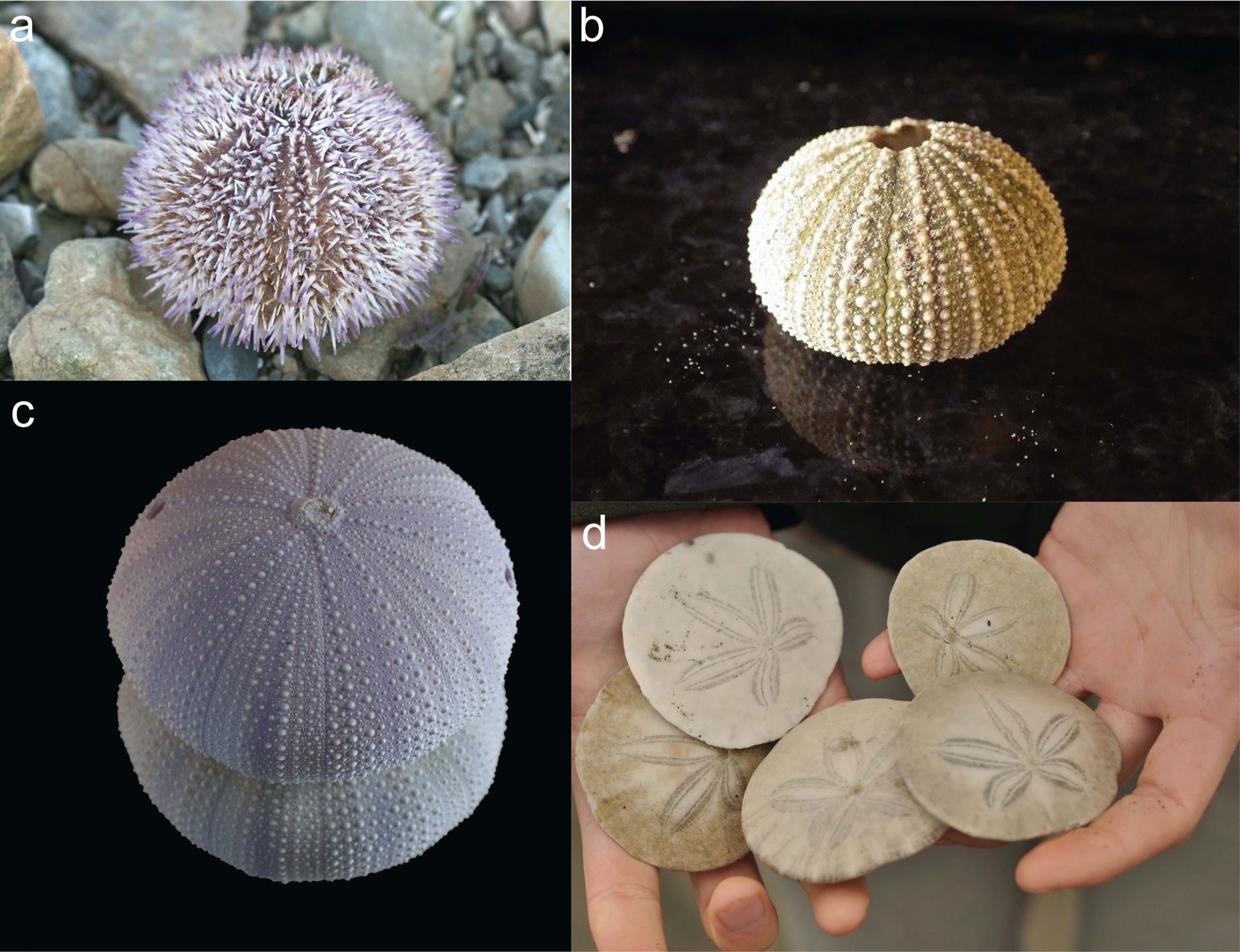
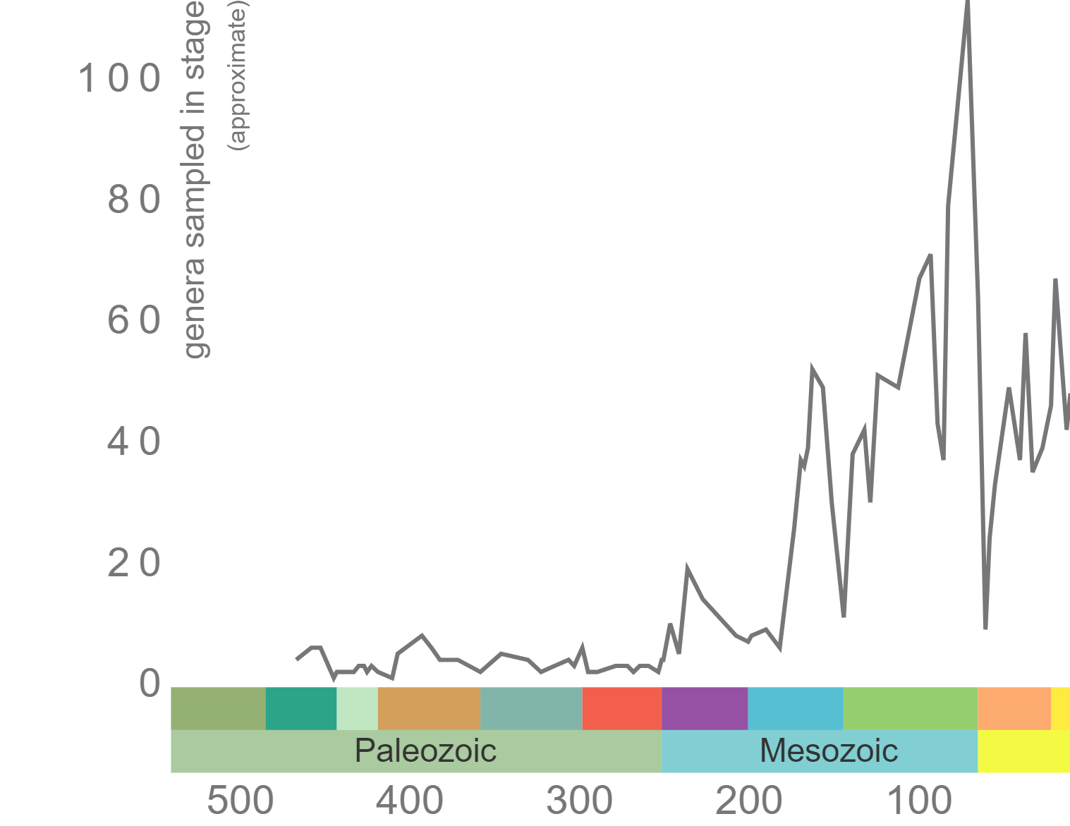
Echinoids first appear in the fossil record in the Upper Ordovician, approximately 460 million years ago, but they didn’t really diversify until the Jurassic (Figure 7.39).
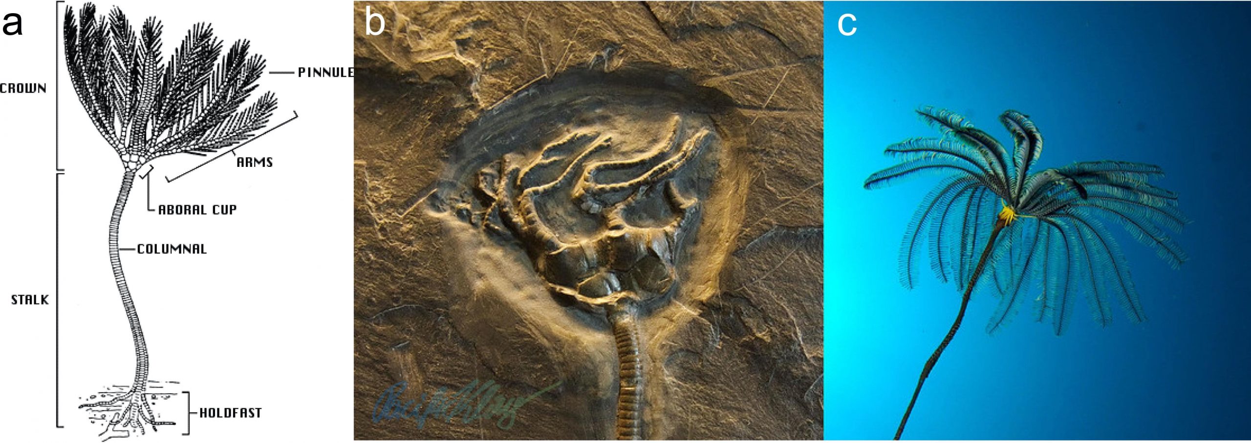
Class Crinoidea
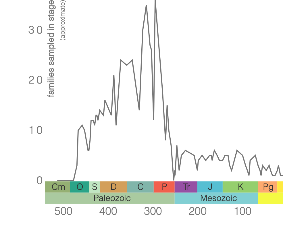
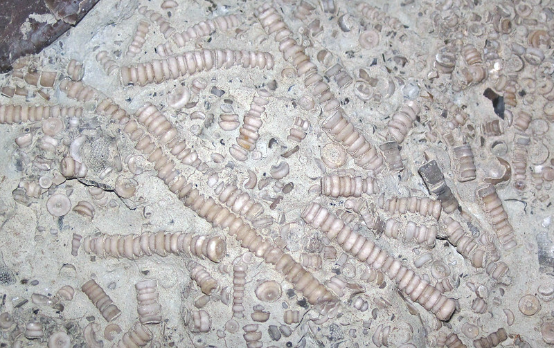
Crinoids, often referred to as “sea lilies,” may resemble plants (Figure 7.40), but they are actually suspension-feeding animals that have been around since the Ordovician (Figure 7.41). They use their arms to catch floating food particles and transfers them to the base of their crown. The crinoid “stem” contains numerous ring-like elements made of magnesium-rich calcite and is held together by a combination of ligaments and muscles. The stem of crinoids is most often found in the geologic record (Figure 7.42). The crown resembles a flower, and this soft tissue is rarely fossilized.
Class Blastoidea
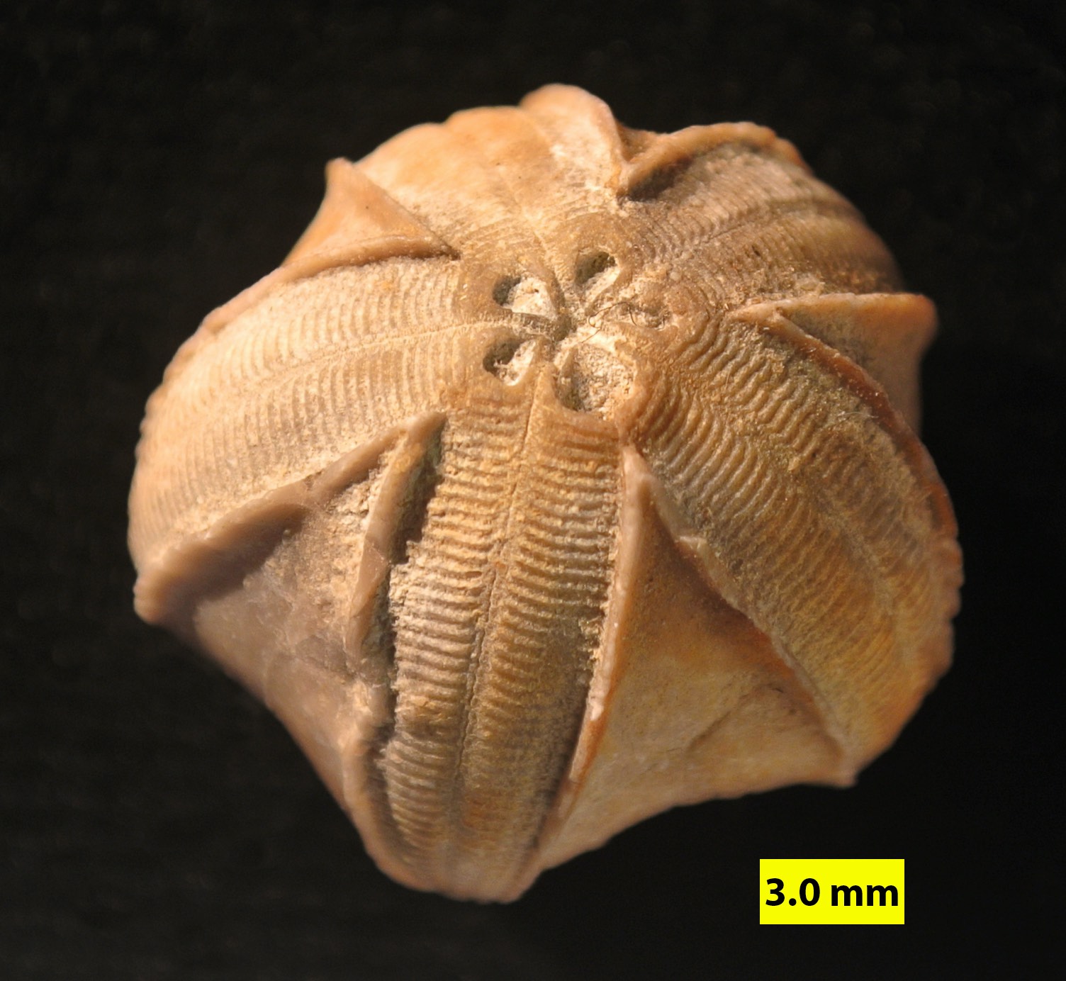
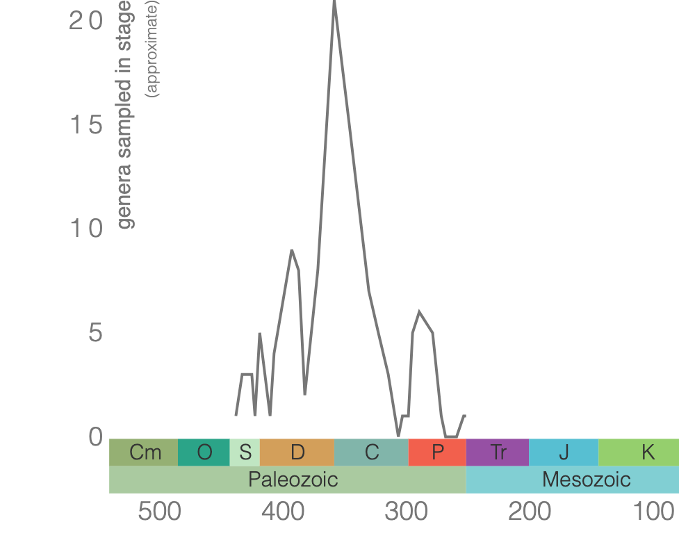
Blastoids are an extinct class of echinoderm. Similar to crinoids, blastoids had a stalk and were suspension feeders. The main body is the theca, which was protected by interlocking plates made of calcium carbonate (Figure 7.43). Blastoids evolved in the Ordovician and went extinct during the End Permian extinction event (Figure 7.44).
Exercise 7.5 – Fossil Identification
To help you identify these fossils, here is a flow chart with some of the observations that may help you decide the phylum and class for the specimens.
- The flow chart has a few blanks. Fill in the blanks with the correct word.
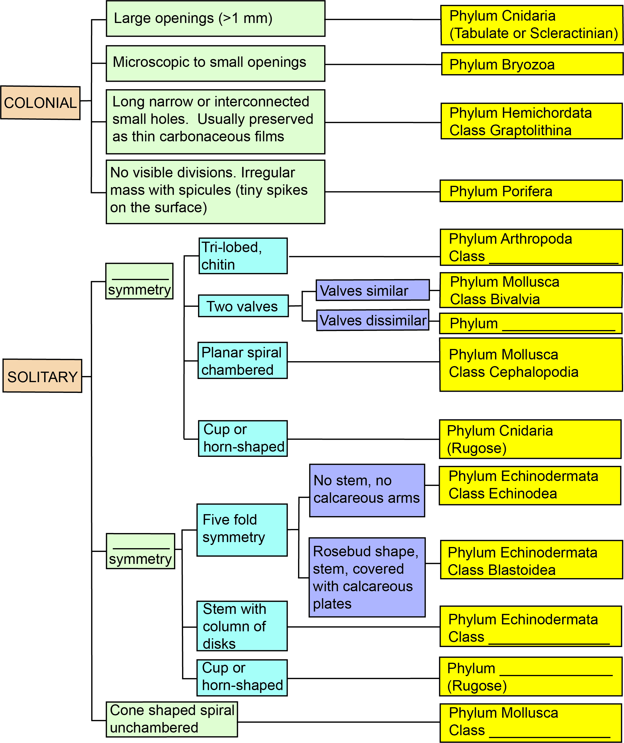
Figure 7.45 – Flow Chart for Fossil Identification. Each color represents different types of observations you should make, with the yellow boxes listing the phylum and class for each type of fossil. You need to fill in a few blanks to be able to use this flow chart. Image credit: VB Sisson. - Your instructor will provide you with a selection of fossils for you to identify. On a separate sheet of paper, make detailed sketches for each fossil from at least two different viewpoints. Be sure to label any identifiable parts and then identify the fossils.
7.10 Extinctions
Over Earth’s history, many species have gone extinct. Extinction is defined as the death of the last individual of a species. You probably already know about the famous extinction event at the end of the Cretaceous that killed all the dinosaurs and many other species. But, have you ever wondered how and when such enormously successful animals went extinct? Are we undergoing a mass extinction right now? If you want to know more, Kolbert (2014) offers a good introduction to extinctions and speculates that the Earth is undergoing a sixth massive extinction, the Holocene extinction event caused by human activity.
Some estimate that 99% of all species (~5 billion species) that ever lived on Earth are now extinct. Massive extinction events are rare, whereas local extinctions are quite common.

Paleontologists postulate that there have been five major mass extinctions in Earth’s history (Figure 7.46); these have had an enormous impact on life by quickly killing large numbers of species from land and sea environments. All of these mass extinctions were caused by major environmental catastrophes. The most famous example was the end of the Cretaceous mass extinction caused by a meteorite that crashed to Earth 65 million years ago. It threw so much dust into the atmosphere that the Earth felt like nighttime for many years, preventing algae, plants, and animals from being able to get enough food to survive. The Late Permian mass extinction was the most devastating of all extinctions. Warming of the Earth’s climate and changes in ocean chemistry caused by the outpouring of basaltic lava in Siberia may have been responsible for this extinction. These two mass extinctions so dramatically affected life on earth that they are used to define the boundaries surrounding the Paleozoic, Mesozoic, and Cenozoic eras.
Exercise 7.6 – Extinction Exercise
The Paleobiology Database (PBDB), an online resource for fossil research, will help you investigate your species extinction. Open the PBDB Navigator. The Navigator page has four parts: 1) The map (in the center) shows continents with dots representing fossil data. The color of these dots represents their geologic age. If you click on the dots, you can see all of the information on each fossil locality and the plants, animals, and other fossil life that occur there. 2) The geologic time scale (on the bottom) shows the major eras and periods (and their subdivisions called stages). If you click on the timescale, the map will show you the location of all known fossil localities from that time interval. 3) The most prevalent taxa (on the right) is shown, such as Mollusca, Brachiopoda, etc. 4) The toolbar (on the left) showing the tools you can use to explore the database. Hover over each tool to see its use. This exercise is inspired by Phil Novack-Gottshall, Benedictine University Evolution of Extinct Animals.
- Select a group of extinct animals you want to study for this exercise. Your instructor may provide this for you. Which group of extinct animals are you studying? ____________________
- On the upper-right corner, type in the name of your extinct group. Next, make a diversity curve for your group by clicking the tool on the left side. You will see a new window show up. The default settings are fine to use. Draw a copy of this graph in the space below.
Sketch Area: - The y-axis plots genus diversity, the number of different genera of animals in the fossil record during each time interval. Describe features of your diversity curve through time. Include features such as when the largest diversity was observed, when your animal group first evolved, and what time period your animal group went extinct? (If your group is not extinct yet, then write that it is not yet extinct.) Did your taxa simply increase in diversity and then suddenly extinct? Or was their evolutionary trends have several periods of increased diversity?
- Some people think extinct animals were evolutionary failures because they are extinct today, or nearly so. Some also claim they were never successful or common animals on earth. Based on the diversity curve, is it fair to claim that your extinct group was a failure? Why or why not? (For comparison, primates have existed for just 16 million years and our species for only 250,000 years.)
- How were your taxa affected by one of the five major mass extinction events in Earth’s history? For each mass extinction, explain whether it (a) had not yet originated, (b) was not affected by the extinction (meaning it did not have a major drop in diversity at this time), (c) was heavily affected by the extinction (meaning diversity drops significantly at this time), or (d) it went extinct before the mass extinction.
- Which mass extinction was the most catastrophic for your group? Explain your answer.
- If your animal group is extinct today, did its extinction occur during a mass extinction? Explain your answer.
Additional Information
Exercise Contributions
Virginia Sisson and Daniel Hauptvogel
References
Evans, S.D., Hughes, I.V., Gehling, J.G., and Droser, M.L., 2020, Discovery of the oldest bilaterian from the Ediacaran of South Australia, Proceedings of the National Academy of Sciences,
Kolbert, E., 2014, The Sixth Extinction: An Unnatural History, Henry Holt and Co., New York City, 319 p.
Leonova, T.B., 2018, Paleozoic Ammonoids: Historical Pathways of the Development of Morphological Diversity, Paleontological Journal, 52, 1746-1755, DOI: 10.1134/S0031030118140113
Miller, A.K., and Furnish, W.M., 1940, Permian ammonoids of the Guadalupe Mountains region and adjacent areas, Geological Society of America Special Paper, 26, 242 pp.
Rohde, R.A. and Muller, R.A., 2005, Cycles in fossil diversity, Nature, 434, 209-210. doi:10.1038/nature03339
Google Earth Locations

a principal taxonomic category that ranks above class and below kingdom
a principal taxonomic category that ranks above order and below phylum
a principal taxonomic category that ranks above family and below order
a principal taxonomic category that ranks above genus and below order
a principal taxonomic category that ranks above species and below family (plural is genera)
a group of organisms that can reproduce with one another and produce fertile offspring
an animal lacking a backbone such as a clam or worm
an object that can be divided into two symmetrical parts across a unique plane, sometimes called a mirror plane
symmetry around a central axis
a body shaped like a sphere arranged around a central point
the uppermost division of the Proterozoic Eon of Precambrian time and latest of the three periods of the Neoproterozoic Era, extending from approximately 635 million to 541 million years ago. Also called Vendian Period
small and microscopic organisms drifting or floating in the sea or fresh water, consisting chiefly of diatoms, protozoans, small crustaceans, and the eggs and larval stages of larger animals
second period of the Paleozoic era, between the Cambrian (~486 Ma) and Silurian (~444 Ma) periods
the fourth period of the Paleozoic era, between the Silurian and Carboniferous periods (405 to 345 Ma)
a wall that divides a cavity into smaller sections
Rib or rib-like structures
the third period of the Paleozoic era, between the Ordovician and Devonian periods (444 to 416 Ma)
a single animal that is part of a colony
the first period in the Paleozoic era, between the Precambrian eon and the Ordovician period (541 to 485 Ma)
these have no front or back end and can move in any direction
these have a definite front and back and move in a particular direction
a cup-like central body with a set of five rays or arms, usually branched and feathery
