
Chapter 5: Stratigraphy
The 2nd edition is now available! Click here.
Learning Objectives
The goals of this chapter are to:
- Evaluate the origin, composition, distribution, and succession of strata to determine past geologic events related to sedimentary environments and tectonic settings
- Apply Walther’s Law to marine transgression and regression
- Reconstruct sediment thickness to understand processes of deposition
- Create stratigraphic columns and correlations using multiple techniques
5.1 Introduction
Stratigraphy is the area of geology that deals with sedimentary rocks and layers and how they relate to geologic time; it is a significant part of historical geology. As you learned in Chapters 2 and 4, one of the primary goals of studying sedimentary rocks is to determine their depositional environment; stratigraphy is no different.
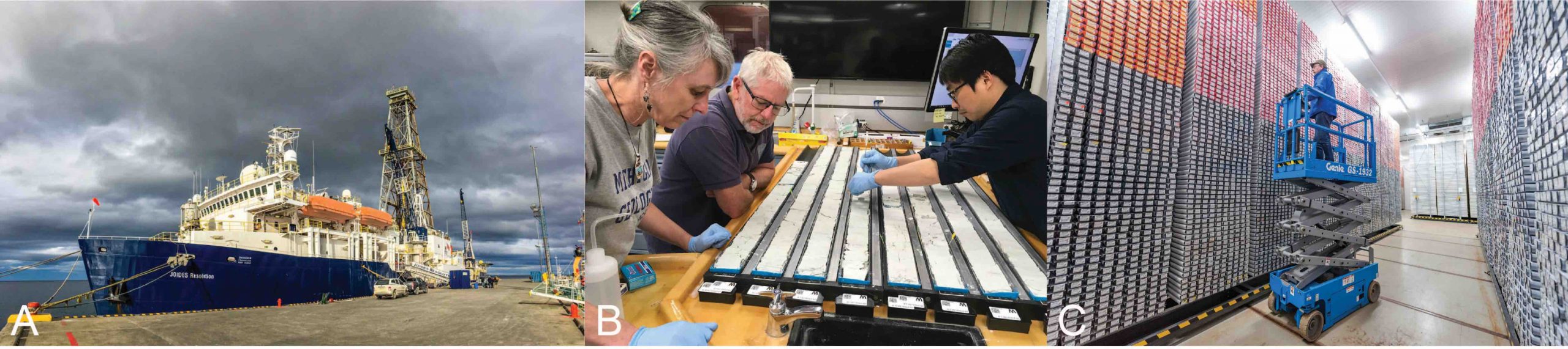
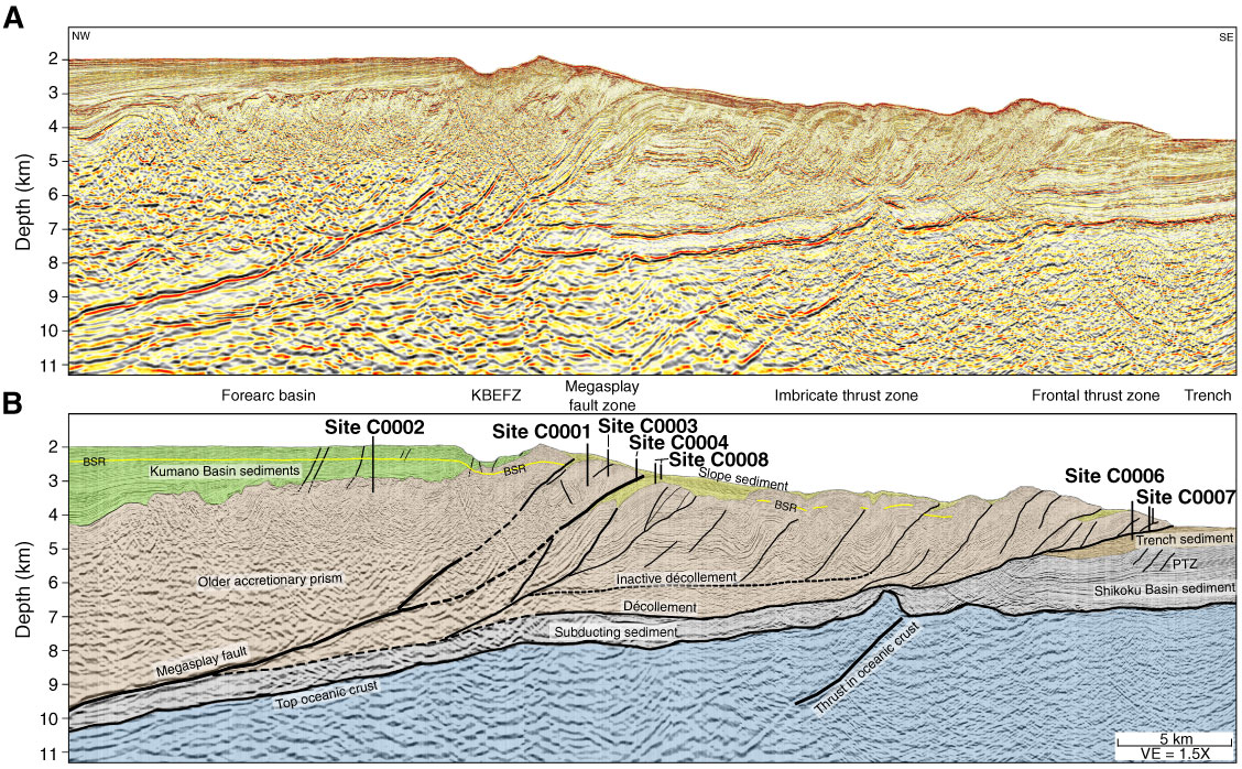
Stratigraphy is mainly studied through outcrop observations, the collection of sediment cores, and seismic surveys. Sediment cores are mostly collected from the ocean floor by organizations like the International Ocean Discovery Program (IODP) using a ship dedicated to drilling (Figure 5.1a). Geologists can then study the collected sediment (Figure 5.1b) or send instruments into the drill hole to measure the geologic properties of the surrounding sediment. The cores are then stored at facilities around the world for scientists to request samples from (Figure 5.1c). Another way to study stratigraphy is to conduct seismic surveys by sending sound waves into the seafloor or ground and monitoring how the waves reflect back to the surface (Figure 5.2). Previous seismic surveys were only collected in a line, but now they are typically collected in grids to get three-dimensional data below the earth’s surface. Geologists use the patterns of reflectivity to help identify the rock types, deformation features, and where there might be water or petroleum and other characteristics in the subsurface. If a seismic survey is repeated over the same area, this gives another dimension of time.
Geologists subdivide stratigraphic columns into formations. A formation is a series of sedimentary beds distinct from other beds above and below and is thick enough to be shown on geological maps. Sometimes several formations are lumped together to form a group. If you want to propose a new formation or group, there are strict guidelines set up by the International Commission of Stratigraphy.
An important tool for stratigraphy is to observe seismic characteristics below the surface. Some call this change in seismic response a seismic facies. Just like grain size is important when describing sedimentary rocks, so are the features in a seismic response. So, when looking at a seismic profile, make observations and ask yourself: Do you see areas without many reflectors? This may be related to its lithology. Are the reflectors continuous? If so, they may be well-bedded. Are they thick or thin? Also, what is their shape – flat or curved?
If you look closely at Figure 5.2, the sedimentary reflectors are relatively flat and show layering in the Kumano Basin (top left side of the image or NW end; highlighted in green in Figure 5.2b) as well as to the right edge to the SE. Layering is flat and parallel to the ocean floor. This pattern implies the sediment was deposited in relatively quiet, low-energy water. Below these regions, and in the middle of the seismic profile, the layering is disrupted and non-continuous; this probably indicates that these sediments were deformed shortly after deposition and before they were lithified as the sediment was scraped off the downgoing oceanic crust. Towards the bottom, the seismic reflectors are very discontinuous as the oceanic crust has no internal structure. The seismic character of the layering lets you know important tectonic and sedimentary history along this profile.
Exercise 5.1 – Sediment Coring and Stratigraphic Columns
This exercise is an analogy for how geologists recover sediment cores. Instead of sediment, though, we will use Play-Doh.
- Using an empty Play-Doh container (or another container), place layers of different colored Play-Doh in the container; don’t use more than 10 layers. These layers of Play-Doh will act as our layers of sediment.
- Take a clear, plastic straw and push it down through the layers of your Play-Doh. This represents geologists drilling into layers of sediment.
- Pull the plastic straw out. You should see all your layers of “sediment” represented in the straw, which geologists recover when collecting a sediment core.
Depending on the type of coring that is done, geologists will split the sediment core in half. One-half of the core will be sampled and studied by geologists, while the other half will be archived and untouched. One of the first things geologists do on a recovered core is describe the lithology. You are going to create a stratigraphic column of your Play-Doh core. A stratigraphic column is a graphical representation of layers of sediment and sedimentary rock and their characteristics. The bottom of a stratigraphic column is always the oldest rock unit in the area.
- Measure and record the total length of your Play-Doh core in millimeters. ___________________
- Measure and record the thickness of each layer in your Play-Doh core in Table 5.1. Start with the upper-most layer.
Table 5.1 – Play-Doh “sediment” layer characteristics Layer Color Thickness (mm) - Now let’s visualize this data by creating a stratigraphic column using Figure 5.3. Start with your uppermost layer, use its thickness to fill in the “Lithology” column. For example, if you measured a thickness of 15 mm, draw a horizontal line at the 15 mm mark. Color your layer so that it matches your Play-Doh. This will be your first layer.
- Now add the second layer to the column. If your second layer is 10 mm, start where the first layer ended and then measure 10 mm down from there. Finish the stratigraphic column with all of your layers.
- If the sediment at the bottom of your column was deposited 100,000 years ago, what is the sedimentation rate of your core in mm/yr? ____________________
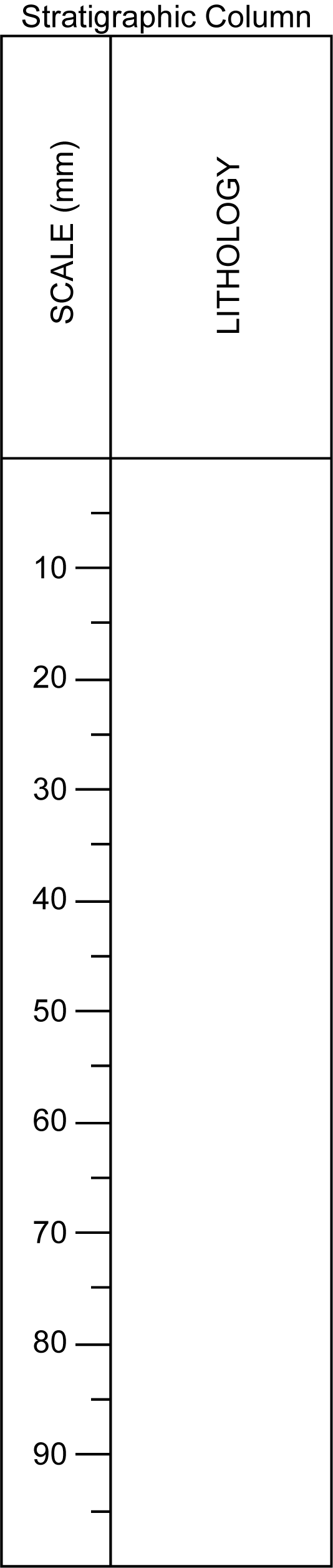
Figure 5.3 – A blank stratigraphic column for Exercise 5.1.
Before you begin the rest of the exercises, you may want to review what you know about classifying sedimentary rocks (Chapter 2) and sedimentary structures (Chapter 4). Remember that clastic rocks are subdivided by grain size, rounding, and sorting. Also, how rocks weather is important in these exercises because their differences in weathering resistance make it easier to see the different stratigraphic units. For example, a fissile shale weathers easily compared to sandstone and limestone.
5.2 Grain Size
One of the simplest analyses done on sediment is a grain size analysis. Remember, clastic sedimentary rocks are classified based on their grain size. It can tell you a lot about the transport and depositional history of the sediment. Some geologists use grain size to help determine the geologic history of the sediment; others use it for studying porosity and permeability to locate fluids (water or oil), or in the case of engineers, how much weight the sedimentary rock can hold before becoming unstable.
Exercise 5.2 – Grain Size
You can try to visually estimate the distribution of grain size in a sample of sediment, but that can lead to significant error if you over- or underestimate something. Visual estimates are best for field measurements, but you need to be more accurate in the lab. Geologists use quantitative approaches with various particle size analyzers (instruments that can accurately measure grain size and shape), but the traditional way to measure grain size was to separate the sediment into different size ranges using sieves and measure their weights. Computerized particle sizers are probably not available for you to use in your lab, so let’s do a grain size analysis on a sample of sediment using sieves.
Note: Grain sizes smaller than 63 μm need to be wet-sieved and dried.
- Measure the starting weight of the entire sediment sample in grams. ____________________
- Now separate the sediment into different fractions using the set of sieves provided by your instructor.
- Measure and record the weight of each size fraction in the first two columns of Table 5.2.
- What weight percentage does each fraction make up? Fill in the third column of Table 5.2. Weight percent is the percentage of the entire weight of the sediment that each size fraction takes up. Take the weight of each fraction and divide it by the total weight, then multiply by 100.
Table 5.2 – Grain size analysis Size fraction range (μm) Weight (g) Weight Percent - Take your weight percent data and plot it as a bar graph in Figure 5.4.
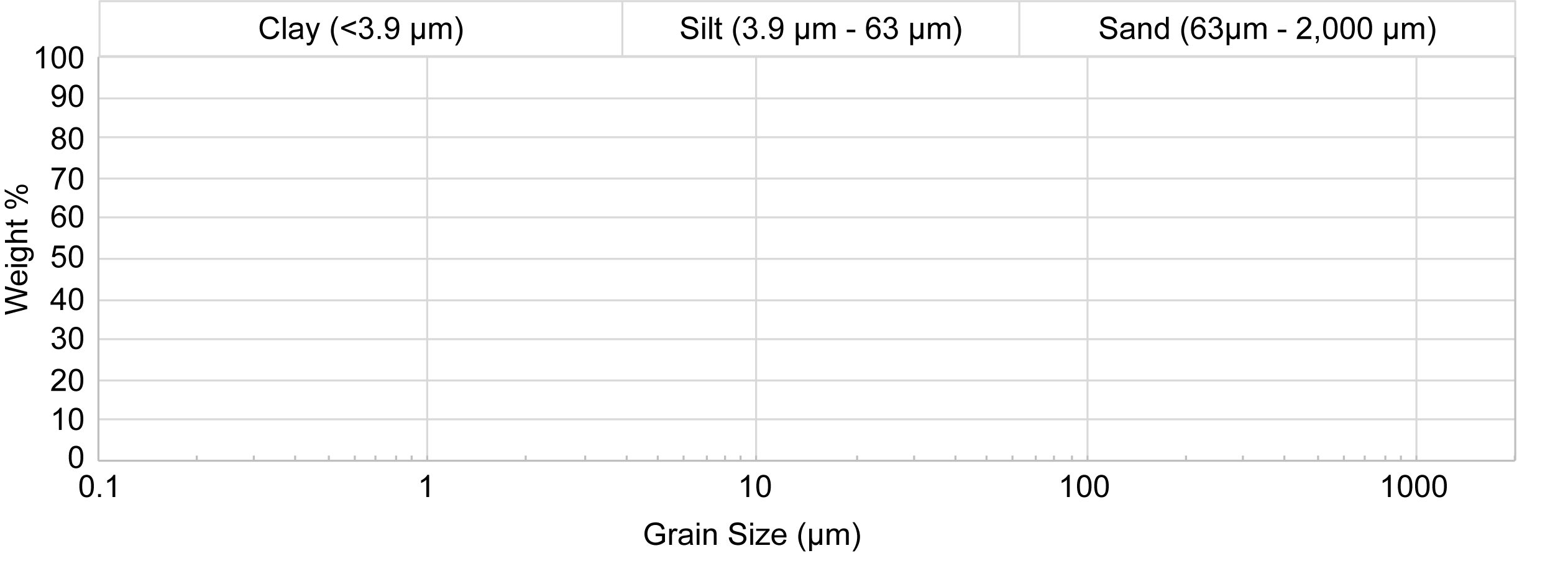
Figure 5.4 – Grain size graph to use in Exercise 5.2. - Another way geologists use sediment grain size is to classify and describe the sediment. Do you remember the triangle (ternary) plot from Chapter 0? Geologists use ternary plots to compare the sand, silt, and clay content of the sediment. Table 5.3 contains percentages of sand, silt, and clay. Plot these percentages on the triangle graph in Figure 5.5 and record the descriptive term for the sediment size in the last column of Table 5.3.
Table 5.3 – Particle size percentages to plot on Figure 5.5 Sand % Silt % Clay % Sediment Description 55 23 22 18 27 55 40 48 12 23 7 70 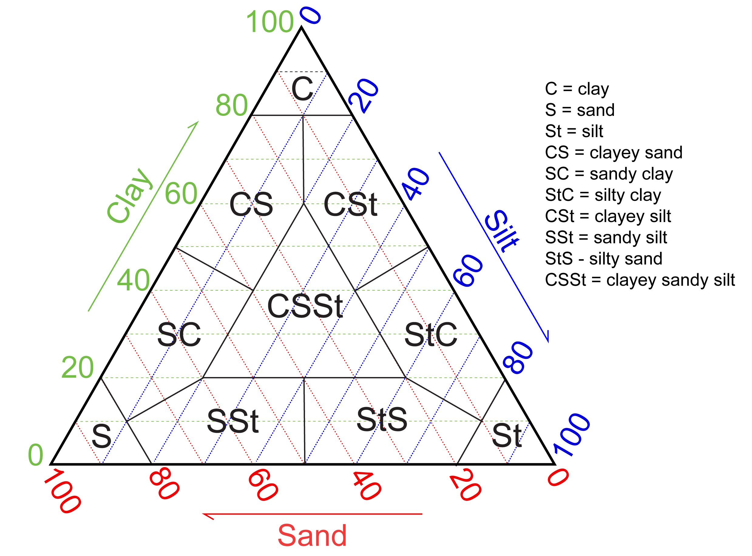
Figure 5.5 – Triangular plot for sedimentary rocks using proportions of sand, silt, and clay. Instructions for how to plot on a triangular plot are given in Figure 0.6. This plot is subdivided into 10 different areas used to assign a rock name to a sample. The abbreviations for each field are given in the figure. Image credit: Adapted from Krumbein, W.C., and Sloss, 1963 by VB Sisson CC BY-NC-SA.
Exercise 5.3 – Interpreting Outcrop Stratigraphy
The boundaries between different geologic time periods are often easy to find in the stratigraphic record as a change in sediment type. Sometimes these correspond to major extinction events. One of these occurs at the end of the Triassic and beginning of the Jurassic time periods (201.3 Ma). At this time, about 25-30% of all marine species died out. The cause for the extinction is debatable, with some geoscientists relating it to increased CO2 in the atmosphere from volcanic eruption of a large igneous province (LIP) in the Atlantic ocean. The Triassic in this region is represented by the Lilstock Formation, deposited in a warm tropical ocean with abundant marine life. Above this is the Blue Lias Formation, well known for its fossil ammonites.
Below is an image created by stitching together many images with software that renders them in three dimensions. Once the image is loaded, you can use your mouse to rotate, tilt, and zoom in on the figure. This image has several numbers that you can click on, highlighting some of the features at the Triassic-Jurassic boundary near Lyme Regis in southern England. There are also two tape measures (inches and feet) draped across the outcrop that you can use to get a sense of the scale of this sea cliff exposure.
- Sketch a stratigraphic column of Figure 5.6. This is easy to do because the limestones and shales weather differently. Limestones tend to be more resistant to weathering than shales and thus make prominent layers.
Sketch Area: - Is there an unconformity in this stratigraphic column? Explain.
- What is the dominant lithology in the Triassic? ____________________
- What is the dominant lithology in the Jurassic? ____________________
- Critical Thinking: Can you explain why the lithology changed?
5.3 Facies and Lithostratigraphy
Lithostratigraphy is a sub-discipline of stratigraphy that deals with the type of rock and depositional environment of sediments and sedimentary rocks. One of the fundamental concepts in stratigraphy is Walther’s Law (Johannes Walther,1860-1937), which states that depositional environments vary in both space and time such that “the facies that occur conformably next to one another in a vertical section of rock will be the same as those found in laterally adjacent depositional environments” (Walther, 1894). That’s a pretty dense statement, so let’s break it down. First, let’s tackle two definitions; facies and conformably. A facies is a characteristic rock that represents a certain depositional environment. These characteristics include physical, chemical, and biological aspects. In geology, sedimentary layers are said to lie conformably when there is no unconformity between them. And remember, sediment is deposited in continuous, horizontal layers.
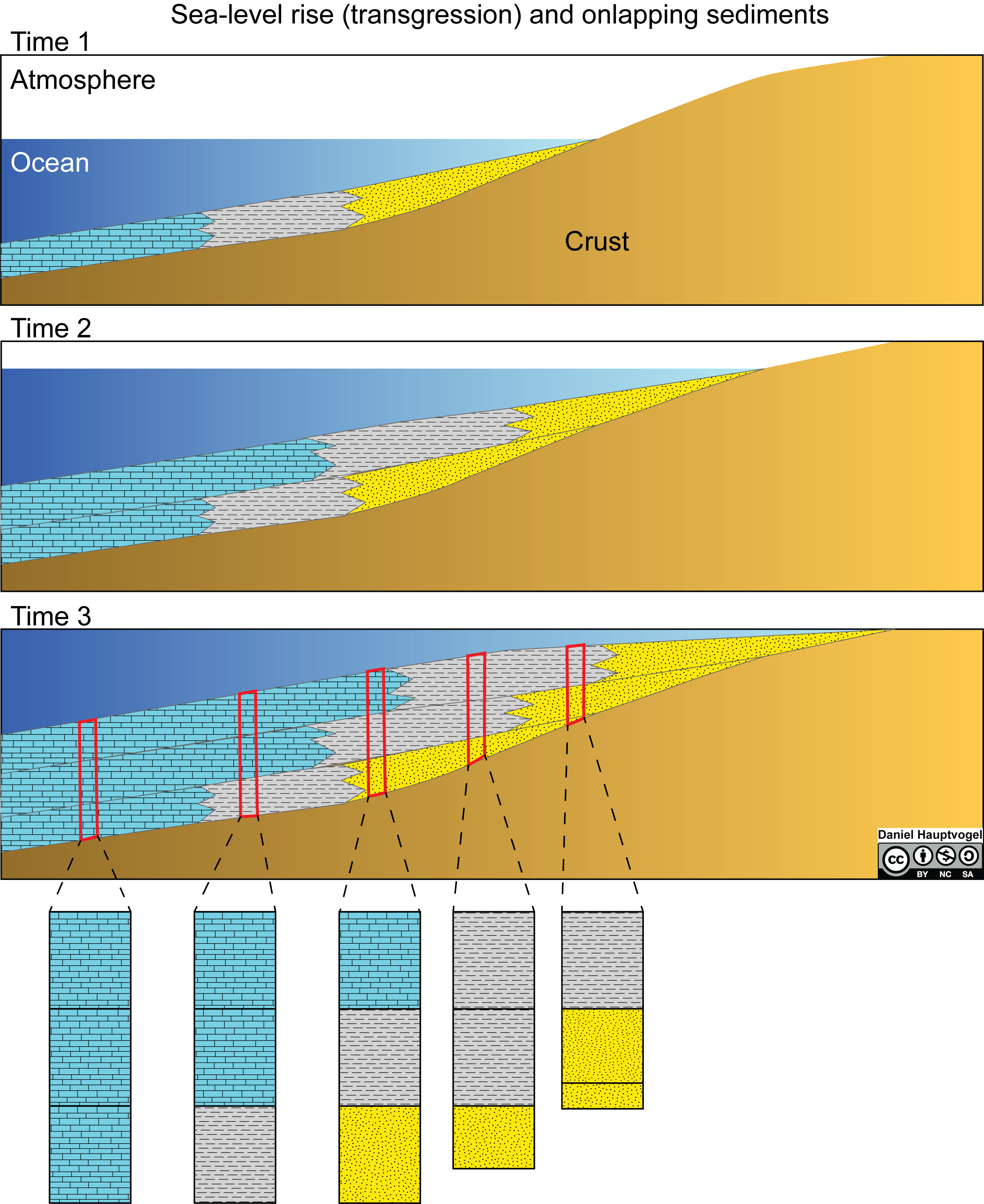
Now for the rest of the law. In the marine environment, sand is deposited close to shore, silt and clay further away, and maybe limestone very far away (Figure 5.7). All three of these sediments are deposited simultaneously and form a single, continuous layer, as in Time 1 in Figure 5.7. The boundary between them is gradational, meaning that the transition from sand to silt, or silt to clay, or clay to limestone is a gradual transition rather than an abrupt boundary (That’s what the zig-zag lines in the figure mean). This gradual transition keeps the single-layer continuous and conformable.
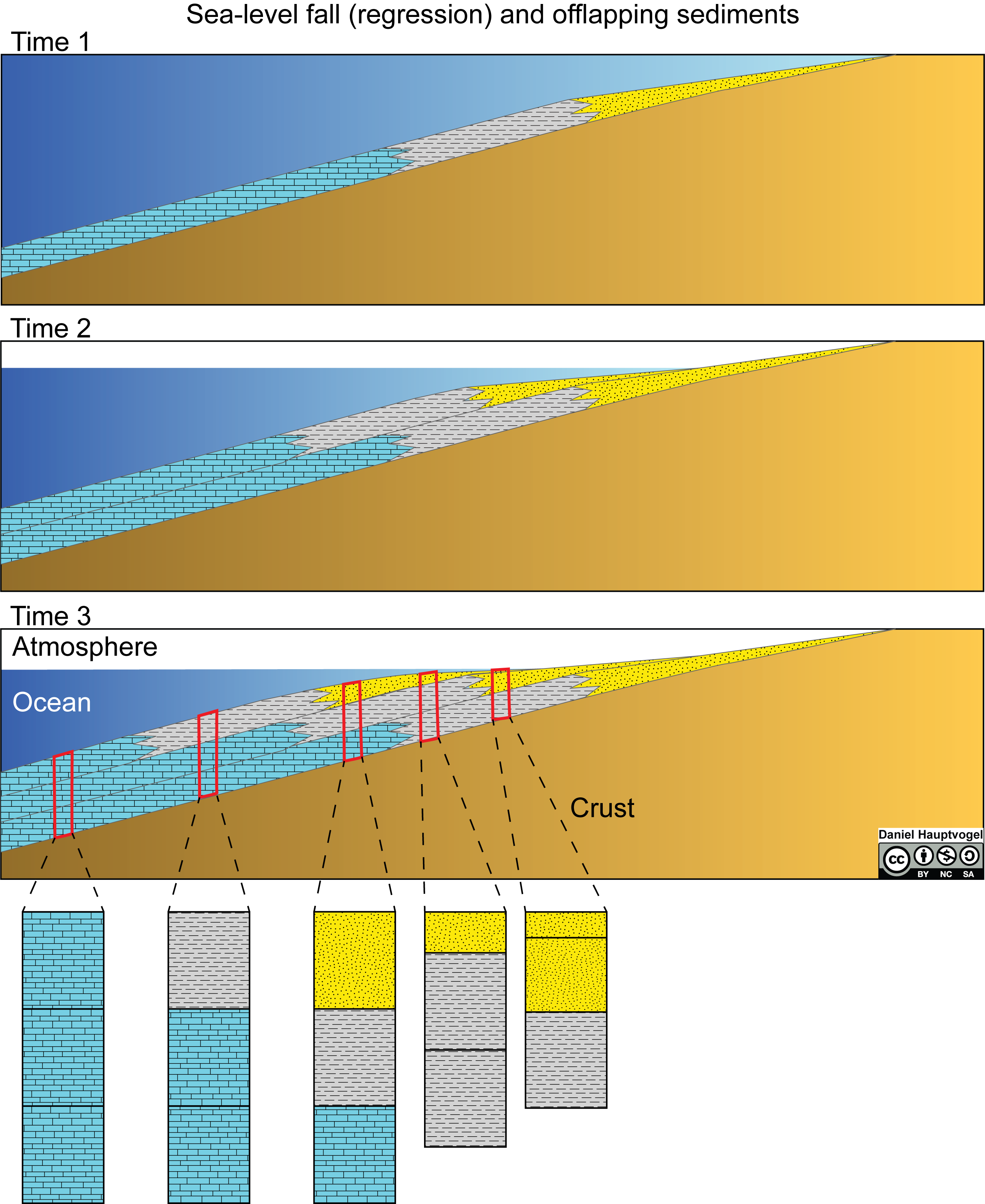
Now, what if sea level were to rise (called transgression), as in Time 2 in Figure 5.7? As the next layer of sediment is deposited, all sediment types are shifted toward the coastline following the sea-level rise. If sea level continues to rise, the next sediment layer will shift even further, as in Time 3 of Figure 5.7. Looking at Time 3 in Figure 5.7, the shale at the bottom is overlain by limestone, and that limestone is the same facies as the limestone to the left of that original shale. The same could be said about the sandstone and shale. That’s what Walther’s Law means, vertical changes in the succession of sedimentary rocks reflect lateral (horizontal) changes in the environment. If sea level were to lower (called regression), the facies would move in the other direction, as in Figure 5.8 (Note: if sea level drops enough to expose sediment, erosion will take place).
Exercise 5.4 – Transgression and Regression
Identifying transgressive (rise) and regressive (fall) cycles in sea level is a key component of lithostratigraphy and sequence stratigraphy. Figure 5.9 is a basic stratigraphic column that contains evidence of transgression and regression.
- Shade in the facies environment box for each layer of sedimentary rock in the column.
- Identify where transgression and regression are taking place. You can mark this with vertical arrows on the side of the figure.
- Can you tell how much sea level has changed? Explain.
- Can you tell what direction the coastline was in? Explain.
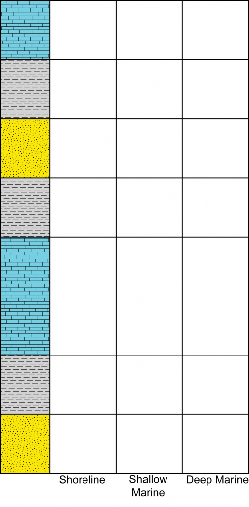
Figure 5.9 – Stratigraphic column for part of Exercise 5.4. The colors and patterns are similar to Figures 5.7 and 5.8. You will need to fill in the columns on the right side of the figure. Image credit: Daniel Hauptvogel, CC BY-NC-SA. - Sedimentary layers are laterally continuous, and they transition into other sediment types. This means that a facies can “pinch out” over horizontal distances. Complete the lithologic correlation in Figure 5.10 below of two sediment cores.
- Which layer pinches out? ____________________
- Explain why that layer pinched out.
- The addition of a second core now lets you interpret the direction of the coastline. Was the coastline to the right or the left? Explain your reasoning.
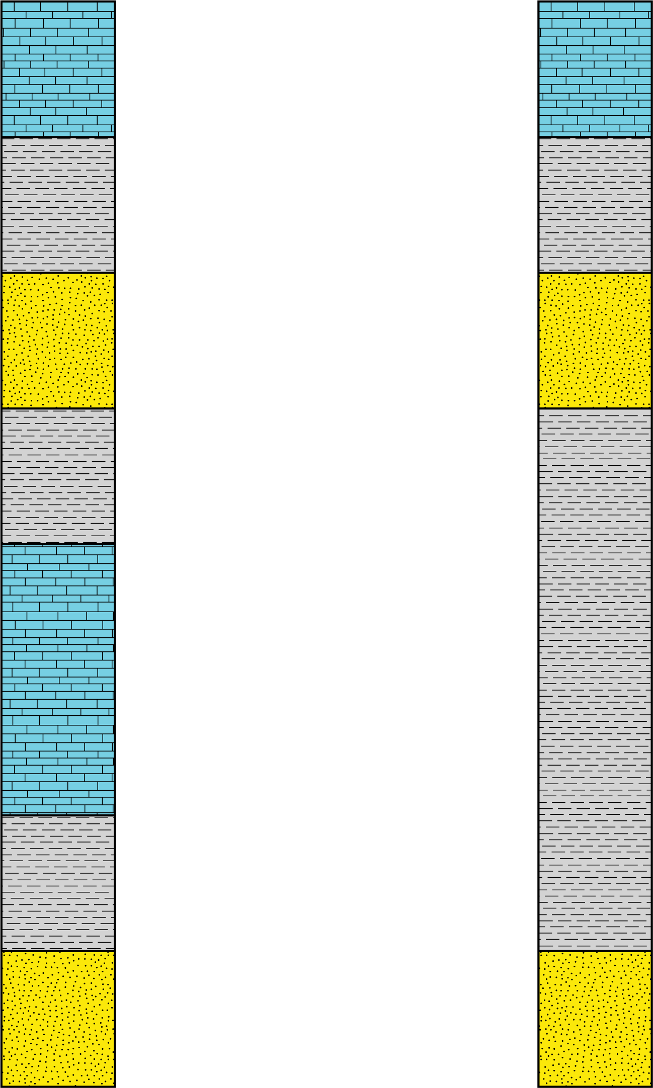
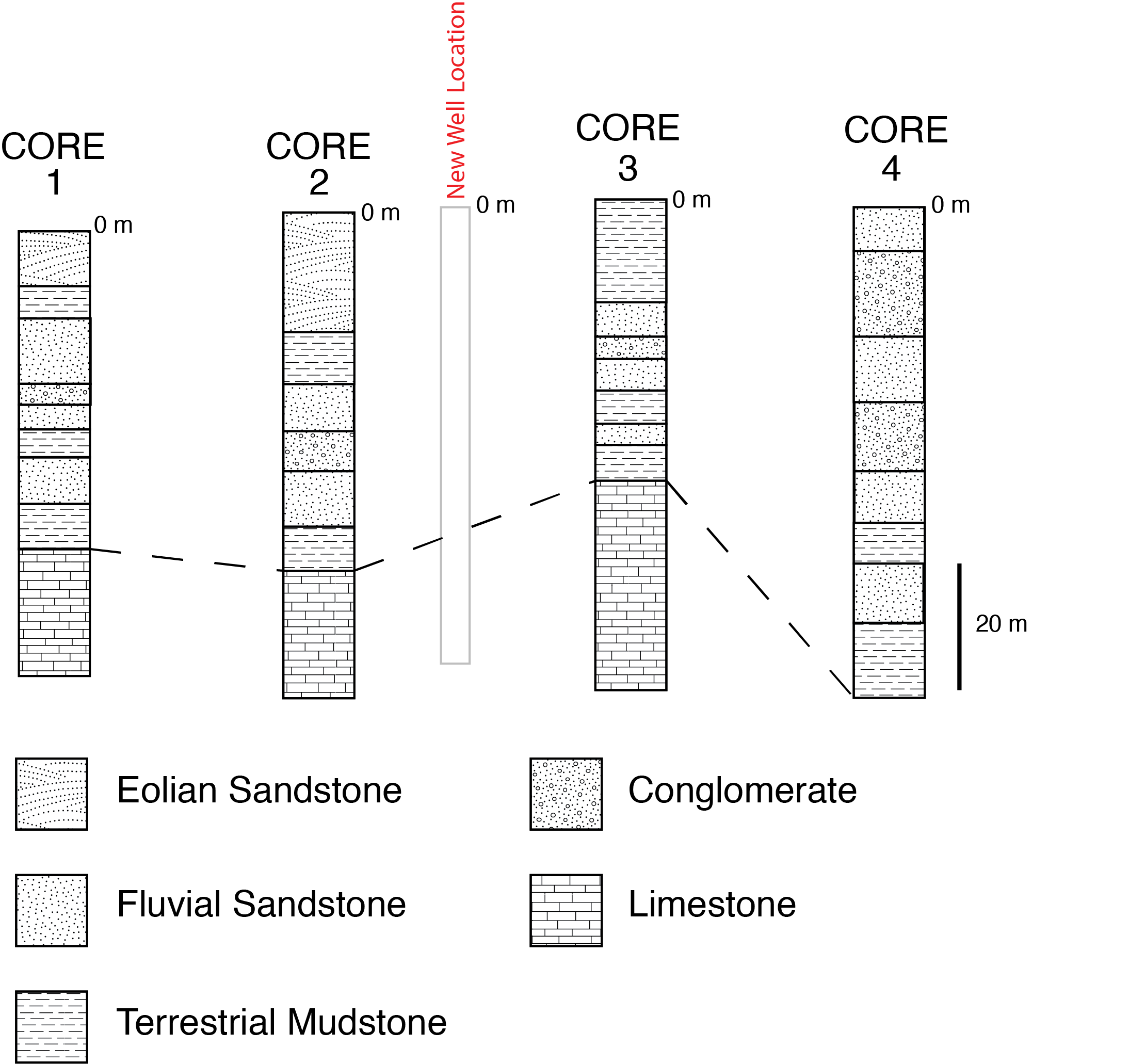
Figure 5.10 – Two stratigraphic columns for part of Exercise 5.4. You will need to correlate the lithology between these two columns. Note, there are no unconformities in these columns. Image credit: Daniel Hauptvogel, CC BY-NC-SA. - Imagine a scenario where you’re working as a hydrogeologist, a type of geologist that deals with water. Your company has assigned you to locate the best source of groundwater for drilling a new water well. Groundwater is contained in rocks with a lot of pore space between the grains. In this area, sandstones make the best aquifers. You have found stratigraphic columns for the rocks in the area from wells drilled on nearby properties. The site you are investigating is located between cores 2 and 3. Use this data to create a cross-section to help you understand the thickness of the various layers and potential reservoirs for groundwater at the new well location. To do this, connect layers with similar lithology, and be careful of layers pinching out. The first layer of limestone is already completed for you.
- Critical Thinking: The best aquifers will be laterally continuous sand layers. Label the layer(s) that you think would be the best source of water.
- Critical Thinking: What is the minimum depth you need to drill to install a new water well? ____________________

Determining facies is an essential part of stratigraphy. In general, there are three main types of facies; marine, coastal, and terrestrial. Many other interpretations of data from sediments and sedimentary rocks rely on an accurate facies analysis. For example, if you are looking at changes in sediment chemistry, they could result from the facies changing. So, you need to have a good and accurate understanding of the facies. You probably discussed rivers and running water in your Physical Geology class. These both erode and deposit sediments. In a meandering river, they can erode their banks and form cut banks or deposit on the opposite shore in a point bar. Further downstream, the sediment transported in the river gets deposited in deltas. Each one of these facies has a distinctive set of sedimentary structures and depending on the velocity of the water a narrow range of grain sizes. Other features of rivers include oxbow lakes, levees, terraces, flood plains, and braided channels. These are all different lithofacies. You may also categorize facies using chemical or biogenic criteria.
Exercise 5.5 – Facies in a Coastal Environment
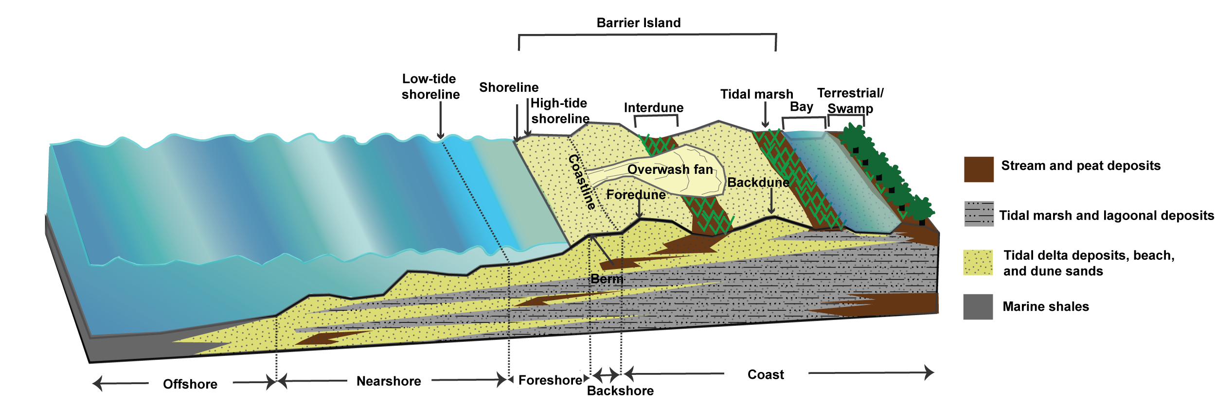
In Chapter 2, you learned about different depositional environments. One environment is coastal which is subdivided into beaches and swamps. Well, beach and swamp environments can be further subdivided based on their proximity to the ocean. These coastal environments can have many sedimentary facies (Figure 5.12), and each has something distinctive about it. You’ll notice that these facies are mainly sandstone or mudstone, which is not distinctive. Sedimentary rocks have other characteristics besides their particle size, including the abundance of fossils, sedimentary structures, and layering patterns of the strata.
- Use Figure 5.12 below to match the environments to the lithofacies and descriptions for: Backshore, Dunes, Foreshore, Bay/Lagoon, Marsh, Nearshore, and Overwash.
| Environment | Lithofacies | Description |
|---|---|---|
| Sandstone | Coarse sand with abundant shell fragments | |
| Sandstone | Medium to fine sand and rare shell fragments | |
| Sandstone | Medium to fine sand and no shell fragments | |
| Sandstone | Fine to very-fine sand, root structures, and cross-bedding | |
| Sandstone with mudstone | Horizontal bedding, root structures, and shell fragments | |
| Mudstone | Bioturbation, root structures, and peat | |
| Mudstone | Bioturbation, root structures, and shell fragments |
- You have collected a 13 m sediment core from the area. Your team has separated and described the sedimentary layers. Based on your team’s descriptions, identify the environment for each layer (using environments from Part I) and fill in the last column of Table 5.5.
| Scale (m) | Lithology | Description | Environment |
|---|---|---|---|
| 0.00 – 0.50 | Sandstone | Coarse sand with abundant shell fragments | |
| 0.50 – 1.20 | Sandstone | Medium sand with occasional shell fragments | |
| 1.20 – 1.90 | Sandstone | Coarse, well-sorted sand with abundant shell fragments | |
| 1.90 – 2.20 | Sandstone | Medium-grained sand with rare shell fragments | |
| 2.20 – 3.80 | Sandstone | Medium-grained sand with rare shell fragments | |
| 3.80 – 4.80 | Sandstone | Medium to fine sand, no shell fragments | |
| 4.80 – 5.60 | Sandstone | Fine sand, well-sorted, cross-bedded with occasional root structures | |
| 5.60 – 7.00 | Sandstone | Medium to fine sand, no root structures or shell fragments | |
| 7.00 – 7.45 | Sandstone | Fine sand, well-sorted with cross-beds | |
| 7.45 – 8.05 | Sandstone interbedded with mudstone | Unconformity at the base, alternating poorly sorted sand and 1 to 10 cm thick beds of silty clay with bioturbation. Root structures and shell fragments throughout. | |
| 8.05 – 8.60 | Mudstone | Silty clay, moderate bioturbation, root structures, shells, and peat | |
| 8.60 – 9.20 | Sandstone interbedded with mudstone | Alternating medium- to coarse-grained sand and 1 to 10 cm thick beds of silty clay with root structures | |
| 9.20 – 10.80 | Mudstone | Silty clay, moderate bioturbation, root structures, shell fragments, and peat | |
| 10.80 – 13.00 | Mudstone | Dark gray silty clay, intense bioturbation, and shells |
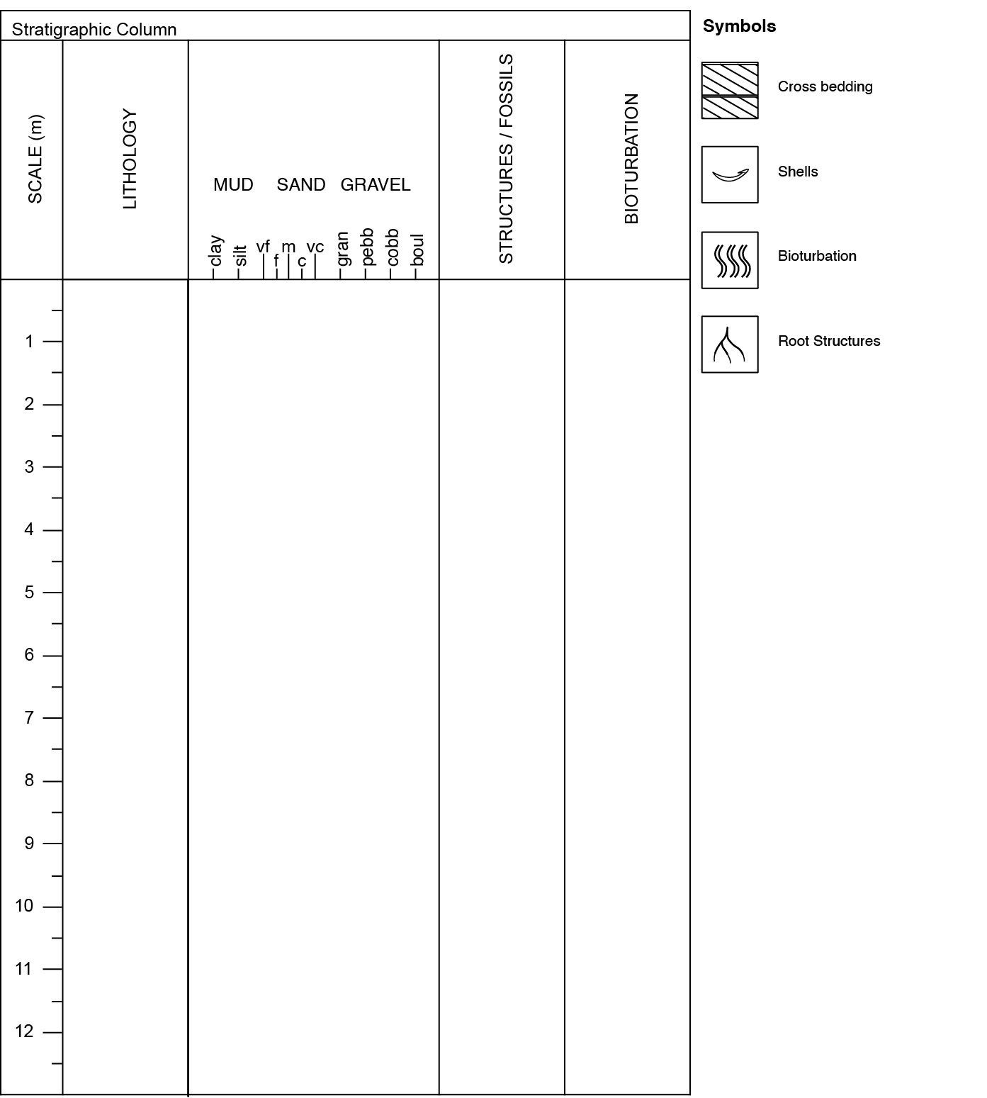
- Use your information to construct your stratigraphic column. If you have computers available, you can do this digitally through the free program Sedlog (Some geologists also use another free program, PSICAT); otherwise, you can use Figure 5.13 to hand-draw your column. Indicate which facies of trace fossil is likely the cause of the bioturbation. Note: a stratigraphic column like this is exactly how geologists present lithologic data from a sedimentary core.
- Geologic History: Briefly describe the geologic history of this core, starting from the oldest layer.
Exercise 5.6 – Facies and Biostratigraphy
Remember that not all stratigraphic units are laterally continuous, which can make correlation difficult. In 1820, William Smith noticed that he would occasionally find fossils while digging canals in different parts of England. He noted that the types of fossils changed according to his location. Whenever he found fossils that matched, he assumed the locations were from the same layer and made maps detailing this. From the maps, he predicted the types of rocks and fossils found at different locations while digging more canals. This made it easy to avoid “problem” rock layers and predict the best way to dig a new canal.
The branch of stratigraphy that uses fossils to determine depositional environments and ages of sediment is called biostratigraphy. In this exercise, you will use a combination of lithostratigraphy and biostratigraphy.
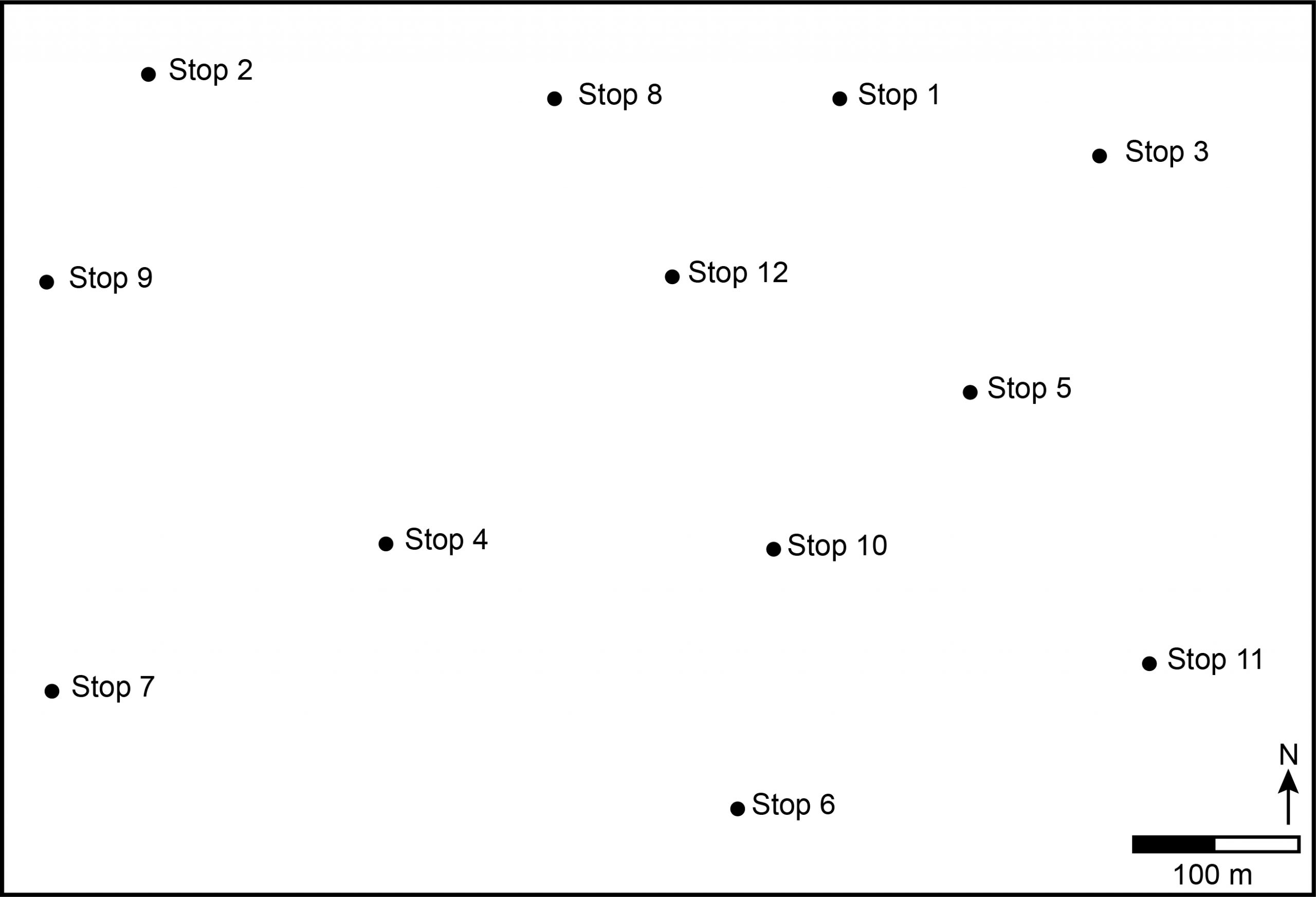
Background: Your cousin has a small fossil shop that is very popular among tourists, but the location where your cousin has been collecting fossil bivalve shells is no longer accessible. He asked you to help find a new place to collect more fossils and to determine its sedimentary environment. Your cousin told you there are 5 different lithologies in the area. You go to a dozen locations (geologists call these stops) and describe the geology at each place.
To help your cousin, you need to create a geologic map. On your map, you need to use colors to differentiate each unit. On geologic maps colors represent the rock age. For example, rocks from the Cretaceous Period are shown in green, and Quaternary deposits are shown in yellow. Each geologic unit is marked with a label. Geologists typically use an abbreviation for the age and name of the formation. For example, in the Grand Canyon, the label Pk refers to the Permian Kaibab Formation and label Mr designates the Mississippian Redwall Formation. A geologic map is usually printed over a topographic base map. Many different types of lines and symbols are found on geologic maps (more on this in Chapter 9). The most prevalent are thin black lines that define the contacts between two different mappable units.
Use your notes from Table 5.6 and the map of the stops in Figure 5.14 to see if you can find a new location to collect more fossils.
- Group the sedimentary rocks from your seven stops into five lithologic units and list these in Table 5.7. Each stop can only belong to one unit.
- On the map in Figure 5.14, draw contact lines that separate the different units. Color each unit according to its geologic age (see Table 5.7).
- Circle an area on your map that you would recommend looking for additional fossils.
| Stop | Description |
|---|---|
| Stop 1 | This is where your cousin used to collect fossils, specifically a shell that looks like a clam. Fossilization has made it dazzling to the eye. |
| Stop 2 | Here there are lots of fossil imprints of leaves and branches. You don’t see any sedimentary structures, and the rock is very dark as well as fine-grained. |
| Stop 3 | This unit is light colored limestone and has some fossil fish. A local geologist has told you that this is the oldest unit in the area. |
| Stop 4 | Cross-bedding! No fossils, but you were fascinated by beautiful cross-bedded sandstone from what look to have been oscillatory waves. |
| Stop 5 | You have found another limestone. There aren’t as many fossil fish here, but you have seen a few smaller ones. |
| Stop 6 | So many shell pieces. Unfortunately, everything here is broken up. There are some fragments of the desired fossil. |
| Stop 7 | A well laminated, dark shale with impressions of fern leaves. |
| Stop 8 | You try to scratch this rock with your geologic hammer but it doesn’t scratch. The grains are well-rounded and well sorted. |
| Stop 9 | A fissile rock that easily breaks when you try to get a sample with your geologic hammer. |
| Stop 10 | A fine grained rock with molds and casts of bivalve fossils and a few gastropods (snails). |
| Stop 11 | This tan fine-grained rock fizzes when you put a dilute acid on it! |
| Stop 12 | Another rock that fizzes when you put dilute acid on it. However, this one has large, angular, poorly sorted fragments. |
| Unit | Stop(s) within unit |
|---|---|
| 5 | |
| 4 | |
| 3 | |
| 2 | |
| 1 |
5.4 Physical Properties
When geologists recover sediment cores, they run an assortment of analyses on the core itself and the hole it came from. After the drilling is completed, geologists will lower an instrument into the hole to take physical property measurements. These measurements can be continuous or occur at specific intervals. Properties that are commonly measured are natural gamma radiation, resistivity, conductivity, density, porosity, and others. These properties are used to give geologists as much information about the rocks or sediment as possible. Physical properties can also be used to correlate sediment cores to each other. Geologists make these correlations to easily compare a section on one core to a section on another.
Exercise 5.7 – Physical Property Correlation
Figure 5.16 below shows the natural gamma radiation logs for two cores recovered by the International Ocean Discovery Program Expedition 369 from the southwestern coast of Australia in the fall of 2017. These two cores were only 20 meters away from each other. The unit for natural gamma radiation is counts per second (CPS). You don’t need the details behind this unit’s meaning, but the higher the number, the more clay particles there are in the sediment (more shale-like). Geologists use this property to determine and compare lithology; sand versus clay and mud. This property is also used extensively both in oil and gas exploration and hydrogeology.
- Correlate the two sediment cores to each other using natural gamma radiation data. Draw dashed lines across both columns that match patterns to each other.
- How many layers did you correlate? _______________
- Compare your answer to b to that of your classmates. Did you have the same number of layers? Explain any differences.
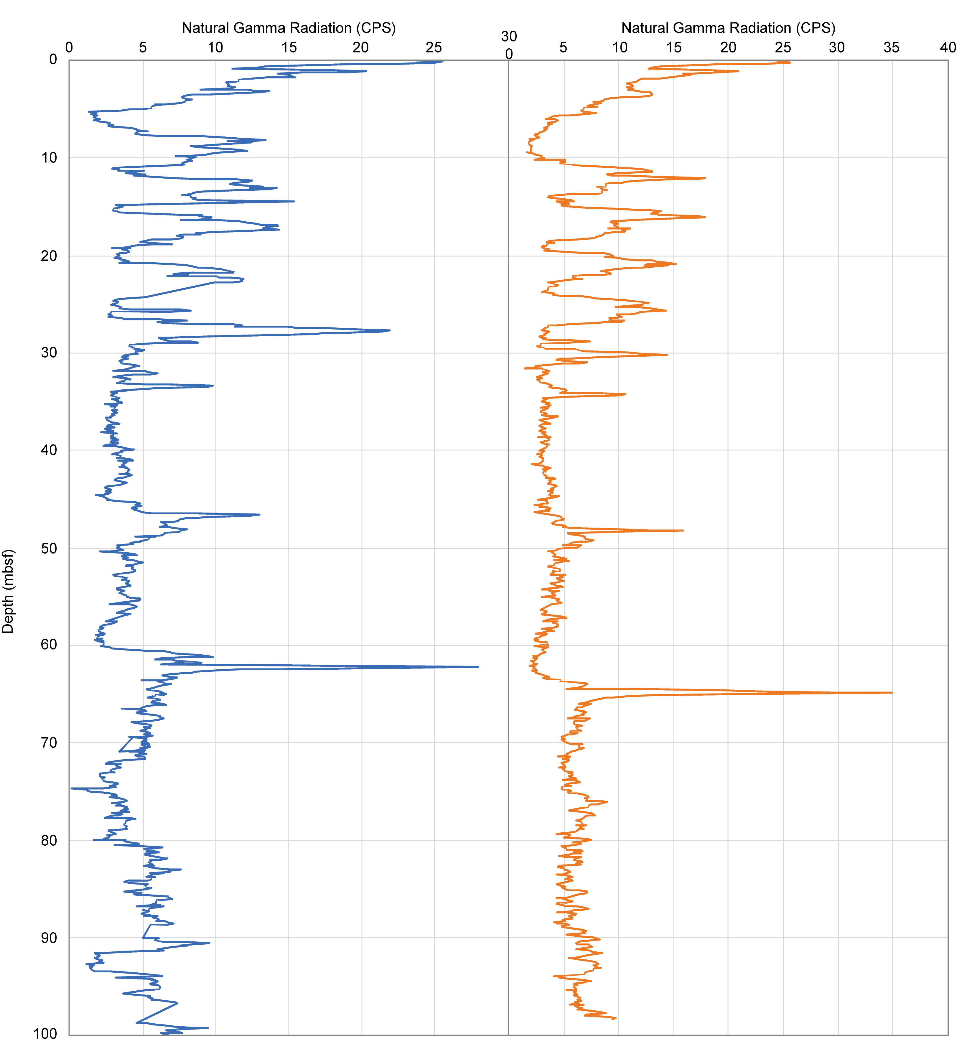
Side note: You might be wondering why the IODP collects sediment cores near each other. The reason for this is that the drill rig is only capable of collecting 1.5 m of core at a time, and when there is a section break every 1.5 m, some of the sediment is actually lost where one section ends, and the next one starts. Additionally, several reasons could cause incomplete recovery of sediment. So, the IODP collects a few cores close to each other and slightly offset to ensure they can get a complete record of the sediment. For example, the first section of the first drill site will start at the seafloor and collect sediment every 1.5 m, but the first section at the second drill site will only go down 1.0 m, and then the rest will be every 1.5 m.
Exercise 5.8 – Paleomagnetic Properties to Determine Depositional Age
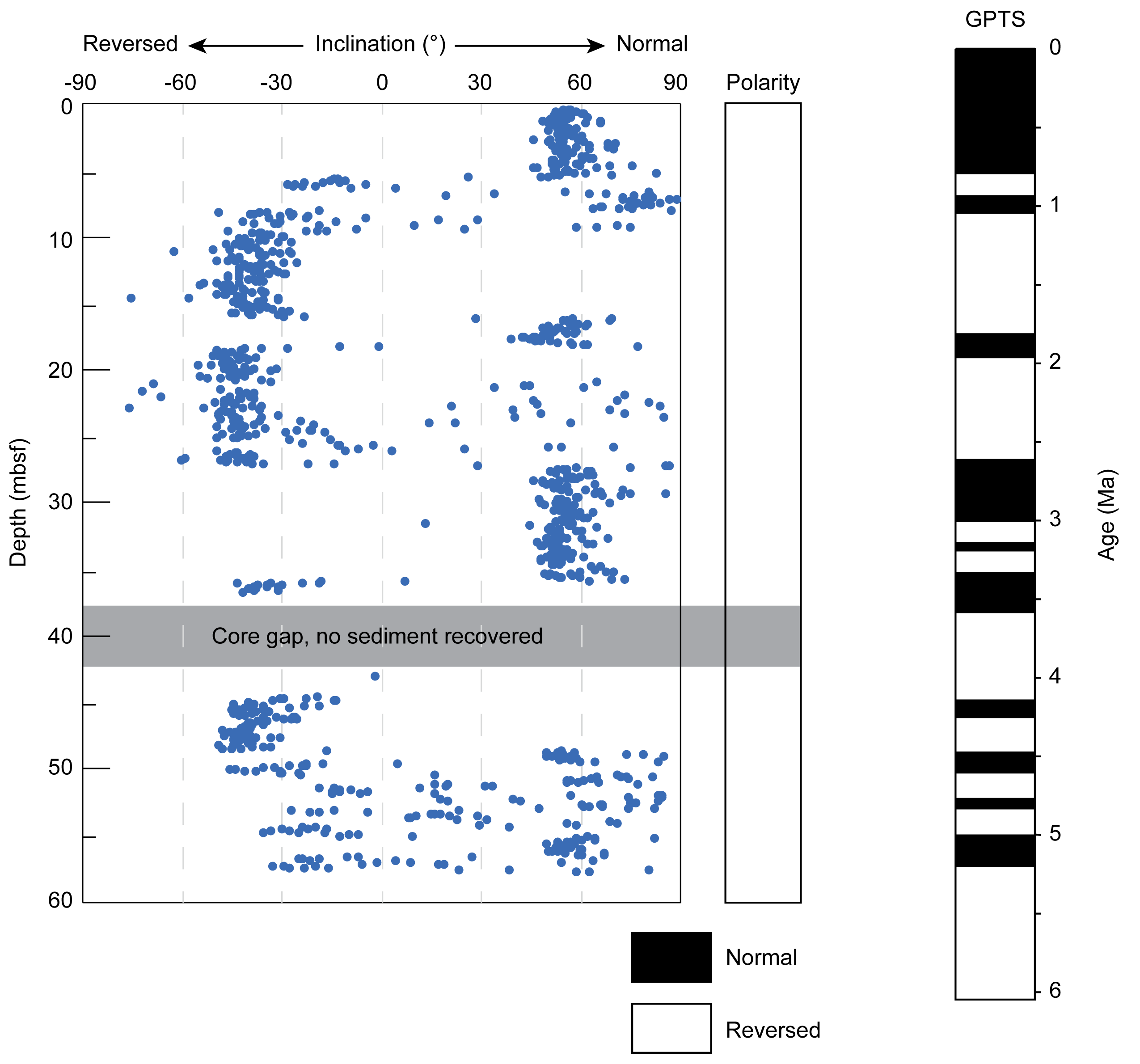
Geologists also analyze magnetic properties of sediment cores for correlation (magnetostratigraphy), but they are also used to help determine the age that the sediment was deposited. Do you remember how magnetic minerals in igneous rocks align themselves to Earth’s magnetic field as the mineral crystallizes? Well, sediments can align themselves while they are being deposited, too. So, paleomagnetic properties in sediment cores can be correlated to known changes in Earth’s magnetic field to determine the sediment’s depositional age.
We currently have normal polarity, where the magnetic north pole and the geographic north pole are in the Arctic. During periods of reversed polarity, the magnetic north pole moves to the geographic south pole in the Antarctic. These magnetic reversals are a natural process on Earth, and geologists have developed a time scale of these reversals called the Geomagnetic Polarity Time Scale (GPTS).
- Use the inclination data from an IODP sediment core in Figure 5.17 to determine periods of normal and reversed polarity. Normal polarity is a positive number, and reversed polarity is a negative number. Fill in the blank polarity column by coloring in the normal polarity intervals in black. Reversed polarity intervals should remain white.
- Correlate your polarity column to the GPTS to determine depositional ages for this sediment core. You can do this by drawing lines that match your polarity intervals of the sediment core to the polarity intervals of the GPTS.
- What is the age range of the missing sediment in the core gap? _________________________
5.5 Seismic and Sequence Stratigraphy
So far, layers on top of one another have been interpreted as being younger than the layers beneath them. In sequence stratigraphy, age is interpreted from lateral (horizontal) variations of rocks based on the sequence of sedimentary strata in sea-level rise and fall cycles. As sea level rises or lowers, sediment deposition migrates landward or seaward. Sea-level regression is interpreted from (clinoforms), which appear to lay somewhat on top of each other at an angle that dips toward the deeper ocean (Figure 5.18). These strata form as land migrates seaward and deposits sediment further away from the original coast. Sea-level rise results in onlapping, where horizontal layers of sediment are deposited against the sloping surface of the clinoforms from the previous sea-level drop. Here is a link to an overview of sequence stratigraphy.
Sequence stratigraphy comes with a slew of new vocabulary words described below and shown in Figure 5.18.
- Base Level – commonly the same as sea level but changes due to basin size and tectonics
- Clinoforms – inclined sedimentary strata tilting toward the deeper ocean
- Downlap – steeply dipping younger strata against a surface or underlying shallowly dipping strata; indicative of sea-level fall
- High Stand – sea level rise and relative increase of onlapping sediment packages
- Low Stand – sea level falls
- Maximum flooding surface – a surface that marks the transition from a transgression to a regression
- Onlap – shallowly dipping, younger strata next to more steeply dipping, older strata; indicative of transgression
- Sequence Boundary – often an unconformity formed by erosion that separates different depositional cycles
- Unconformity – surface separating older from younger rocks and representing a gap in the geologic record
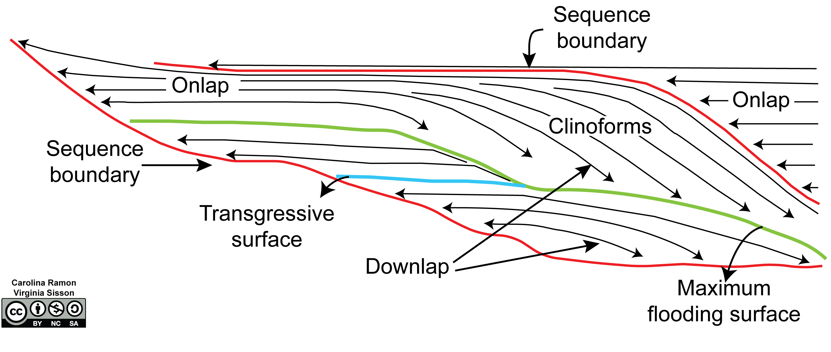
As you look at this figure, there are several things to note. First, clinoforms are not flat. Why you might ask yourself. Well, sediments that are deposited on flat surfaces are flat-lying, whereas those that are deposited on shallowly dipping surfaces are shallowly dipping. New sedimentary layers will mimic the underlying layers until the underlying surface’s angle exceeds that of the maximum angle of repose. The angle of repose is the angle at which loose sediments will cascade or landslide down the slope, and it varies depending on the sediment; sandstone is about 30°, and shale is higher than 40°. So, the slope of the clinoforms reflects the underlying sloping strata. Continental margins are where you can commonly find sloping surfaces.
Look carefully at the top sequence boundary. Does it look like a clinoform? Sometimes sequence boundaries look similar to clinoforms as the transition between depositional cycles can be very gradual without significant erosion. You have to look closely to see if there is onlap of the next strata to distinguish a clinoform from a sequence boundary.
Exercise 5.9 – Sequence Stratigraphy from a Seismic Image
In this exercise, you will work on determining whether sea level influenced the deposition of Cretaceous sediments as well as the different features associated with sequence stratigraphy. To do this, you will investigate a stratigraphic section in the Colville Basin, Arctic Alaska (Figure 5.19).
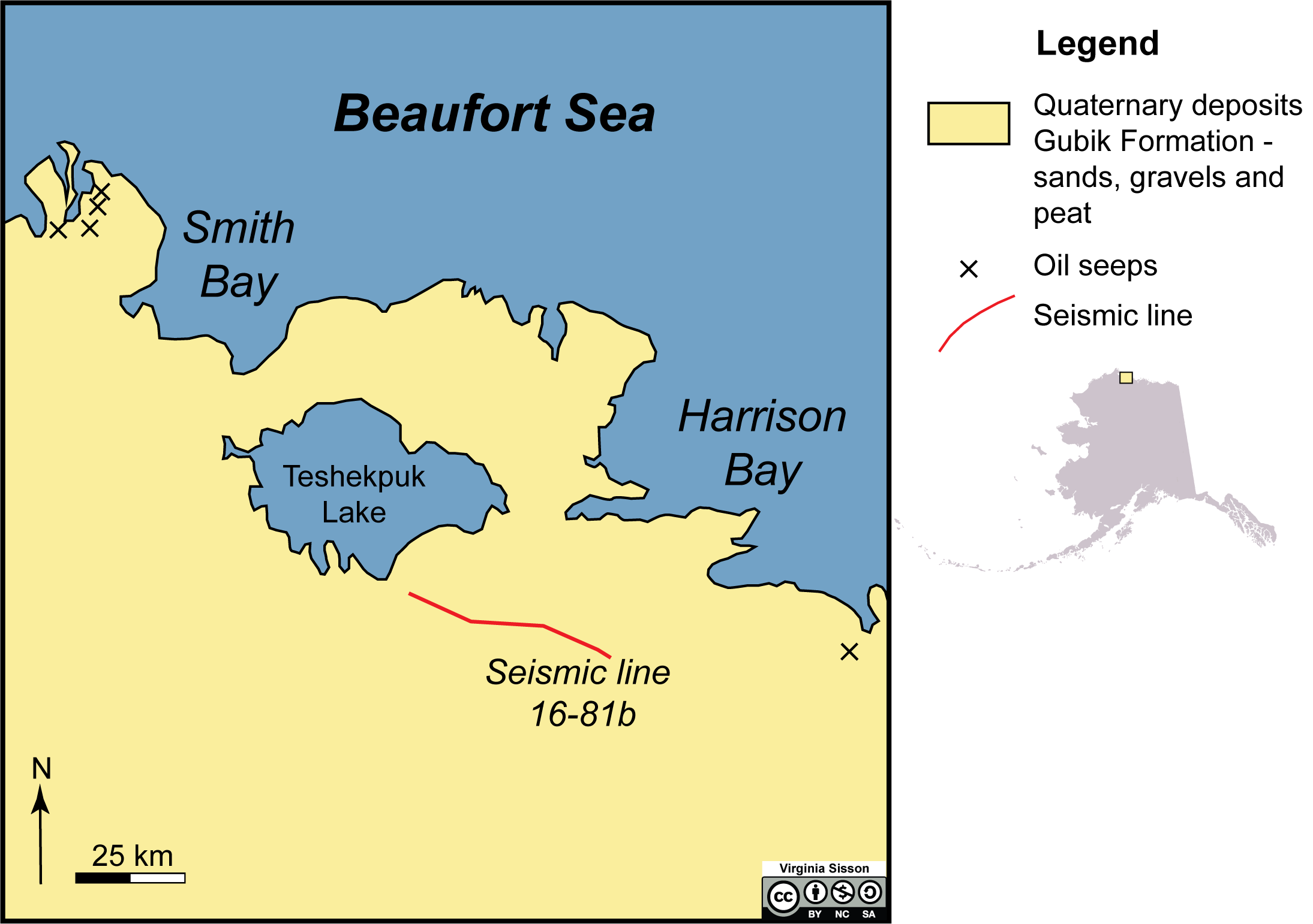
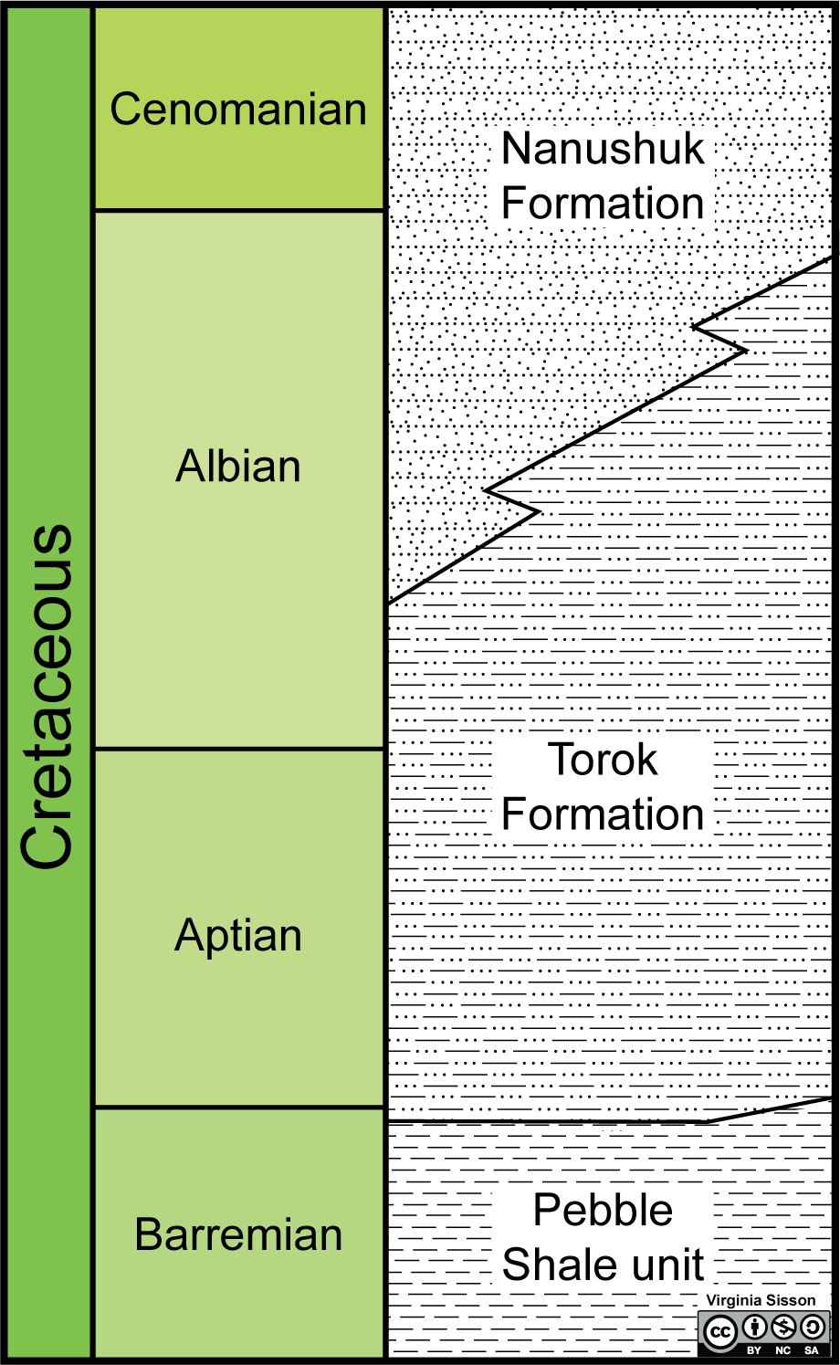
Long before Alaska was granted statehood, oil was found seeping from the ground in the Arctic. This oil helped lead to creating the National Petroleum Reserve of Alaska (NPRA – an area the size of Indiana). This area is also known for its coal; some have estimated that this region has ~40% of the U.S. reserves. Arctic Alaska has provided much of the energy resources for the rest of the United States for many years. To help define where the oil was located and how it formed, the U.S. Geological Survey conducted many seismic surveys (often called lines) across the region. We will look at one line for this exercise. Figure 5.20 shows the Cretaceous formations in this section: Pebble Shale unit, Torok Formation, and Nanushuk Formation.
Before you analyze the seismic section, you should know how sea level is changing worldwide. If you know if the sea level was rising or falling during sediment deposition, this will let you know if you are in a highstand or lowstand environment.
- We don’t know the exact age of these sediments, so first, you must determine the absolute age of these formations using Figure 3.1. Fill out the ages in Table 5.8.
Table 5.8 – Worksheet for Exercise 5.9a Rock Formation Absolute Age Range Nanushuk Formation Torok Formation Pebble Shale unit - Use the ages you determined in a and the sea-level record for the Phanerozoic Eon in Figure 5.21 to determine if sea level was rising, falling, or not changing when these three formations were deposited. You might wonder how to do this since this figure has three different sea-level curves. It’s up to you to choose one of these to answer this question. Indicate which curve you used to answer this question.
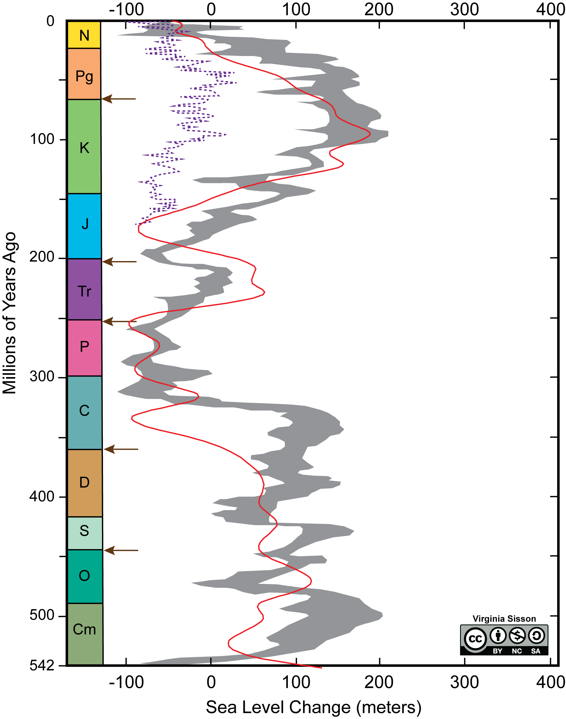
Figure 5.21. Three proposed sea-level curves for the Phanerozoic Eon. The gray area is a compilation of curves proposed by researchers at ExxonMobil. The dashed purple curve considered global ice volumes without tectonic influences on accommodation space. The red curve used a geodynamic model combined with sea level data. Image credit: Simplified by Virginia Sisson CC BY-NC-SA from Vérard et al. (2015). - In this exercise, you will identify the age progression of deposition and the different features associated with sequence stratigraphy. In the seismic image (Figure 5.22), identify as many clinoforms as you can. Number them in order of depositional age, with “1” being the oldest. You should be able to identify at least 10 clinoforms. Hint: There is at least one unconformity. Pay attention to the angles at the beginning and end of your features and the angle at which they touch another reflector; if it is at a high angle, this is likely to be either onlap or downlap.
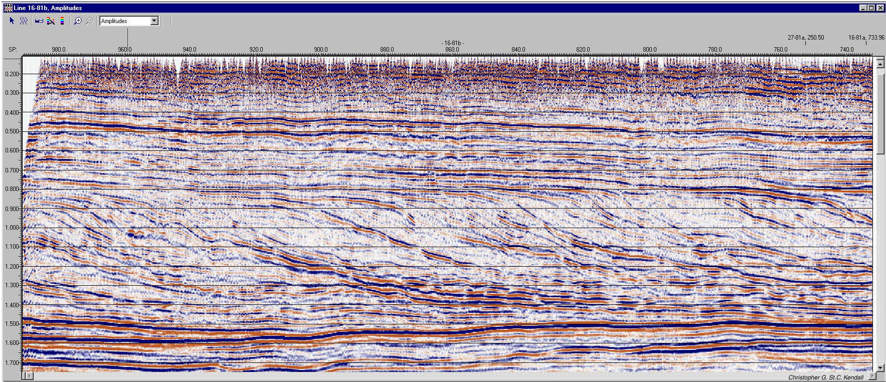
Figure 5.22 Seismic cross-section (line 16-81b) across Cretaceous sediments of the northeastern National Petroleum Reserve of Alaska (NPRA). These sediments filled the Colville foreland basin about 6000′ deep. This view is looking to the north so that the left side is to the west, whereas the right side is to the east. Figure 5.19 shows the location of this seismic line. Blue is for positive amplitude, black for negative amplitude, and white is for no amplitude difference. Image credit: SEPM exercises for sequence stratigraphy with data from U.S. Geological Survey NPRA data archive public domain. - Using the seismic features as your guide, which direction would you go to find a marine basin? Explain your reasoning.
- Based on the seismic section, do you think that sea level was rising or falling during the deposition of this sequence? Explain your reasoning.
- Critical Thinking: Is your answer to e the same or different from your answer to b, which used the stratigraphic section and the global sea-level curve? If it’s different, explain what might cause the discrepancy. Or, if your answers are the same, how does this strengthen your interpretation?
All the previous exercises were aimed at understanding changes in stratigraphy due to environmental conditions and processes. Another component of stratigraphy is the tectonic setting for the sedimentary basin. So, which two tectonic settings are important to consider? The next two exercises will address both convergent and divergent plate boundaries in terms of stratigraphic change. Transform margins may have overlapping faults that create subsidence and small pull-apart basins.
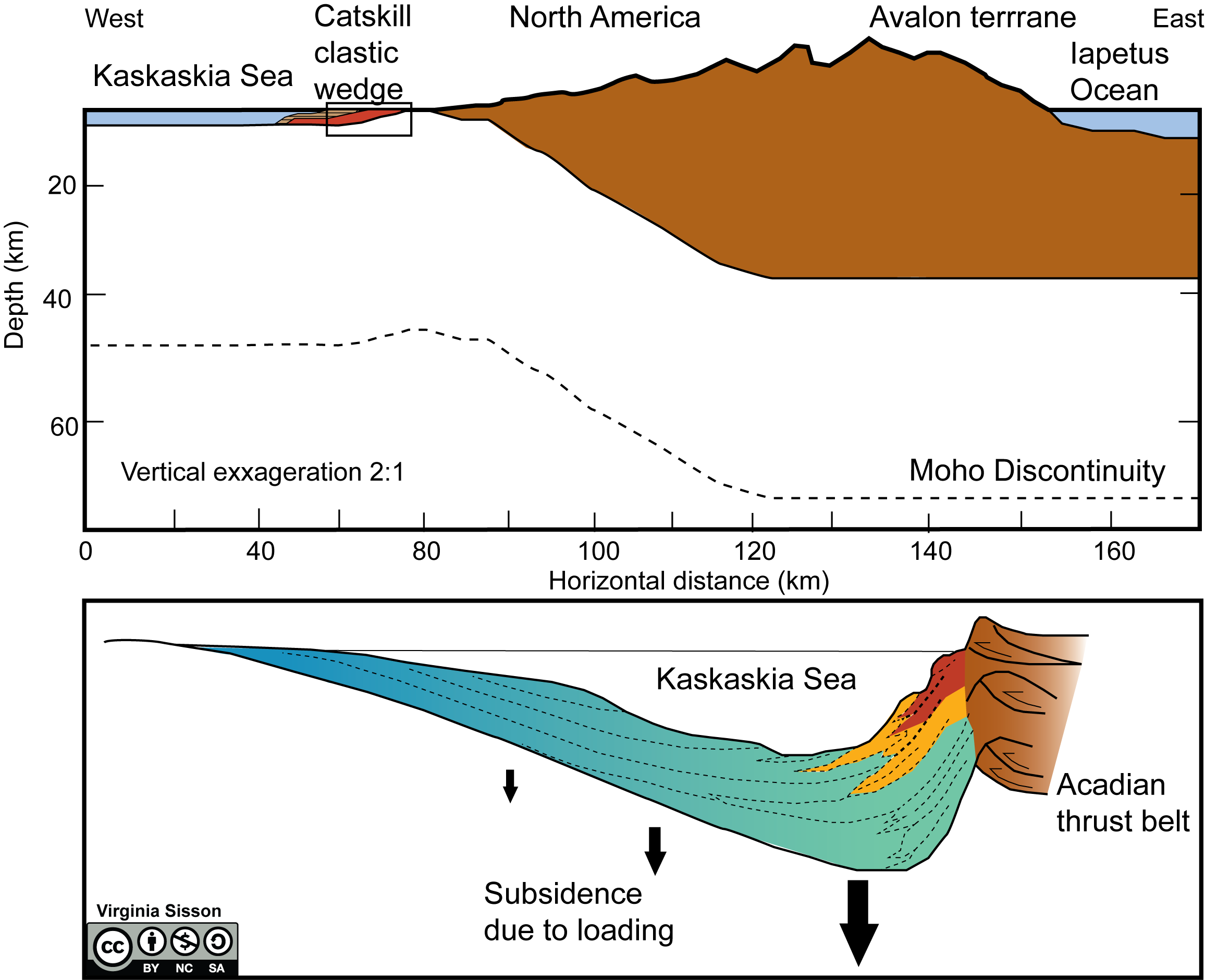
The Appalachian/Caledonide Mountains formed during three separate tectonic events over a period of 220 million years. These events were the Taconic (470 to 440 Ma), Acadian (420 to 380 Ma), and Alleghenian (350 to 250 Ma) orogenies. Between each of these tectonic events, the mountains eroded as they were uplifted. One of the concepts you need to know for this exercise is the effect of increasing the weight on the lithosphere. You may have learned about isostasy in Physical Geology and how the lithosphere responds like an iceberg melting in the ocean. Well, during continental collision, the added weight of the continental mass will cause the lithosphere to bend, creating a foreland or foredeep basin. For example, the Persian Gulf is a basin formed from the collision of the Asian and Arabian plates creating the Zagros Mountains. These sedimentary basins often form shallow (30-100 m) repositories for continentally derived sediments. If the area beside the continental collision is wide, it will form a shallow inland ocean (sometimes called an epeiric or epicontinental sea), such as Baffin Bay in northern Canada.
Exercise 5.10 – Convergent Tectonics in a Sedimentary Record
The Catskill clastic wedge (Figure 5.23) is a Devonian sediment package sourced from the Appalachian Mountains during the Acadian Orogeny. This sediment package extends from New York through Virginia and West Virginia and is part of the larger Appalachian Basin. In western Virginia and eastern West Virginia, the Catskill clastic wedge contains evidence for three phases of the Acadian Orogeny:
Phase 1 – A rapid drop of the seafloor caused by the massive weight of the mountains. The load causes the lithosphere to bend, creating a concave basin in front of the uplifting mountains. It is characterized by a sudden change to deep-water sediments such as shales.
Phase 2 – As the mountains erode, coarse sediment is deposited. These can be deposited in fluvial (rivers) or near-shore marine depositional settings.
Phase 3 – At the end of the mountain building process, there is a return to a stable passive margin sequence ranging from fine sediment deposition to shallow marine carbonates.
Complete the following questions about the Catskill clastic wedge:
-
- Figure 5.24 is a roadside outcrop of the Brallier Formation in Pennsylvania, composed of shale and fine sandstone layers. Provide a sketch of this outcrop and identify the layers of sandstone vs. the layers of shale.
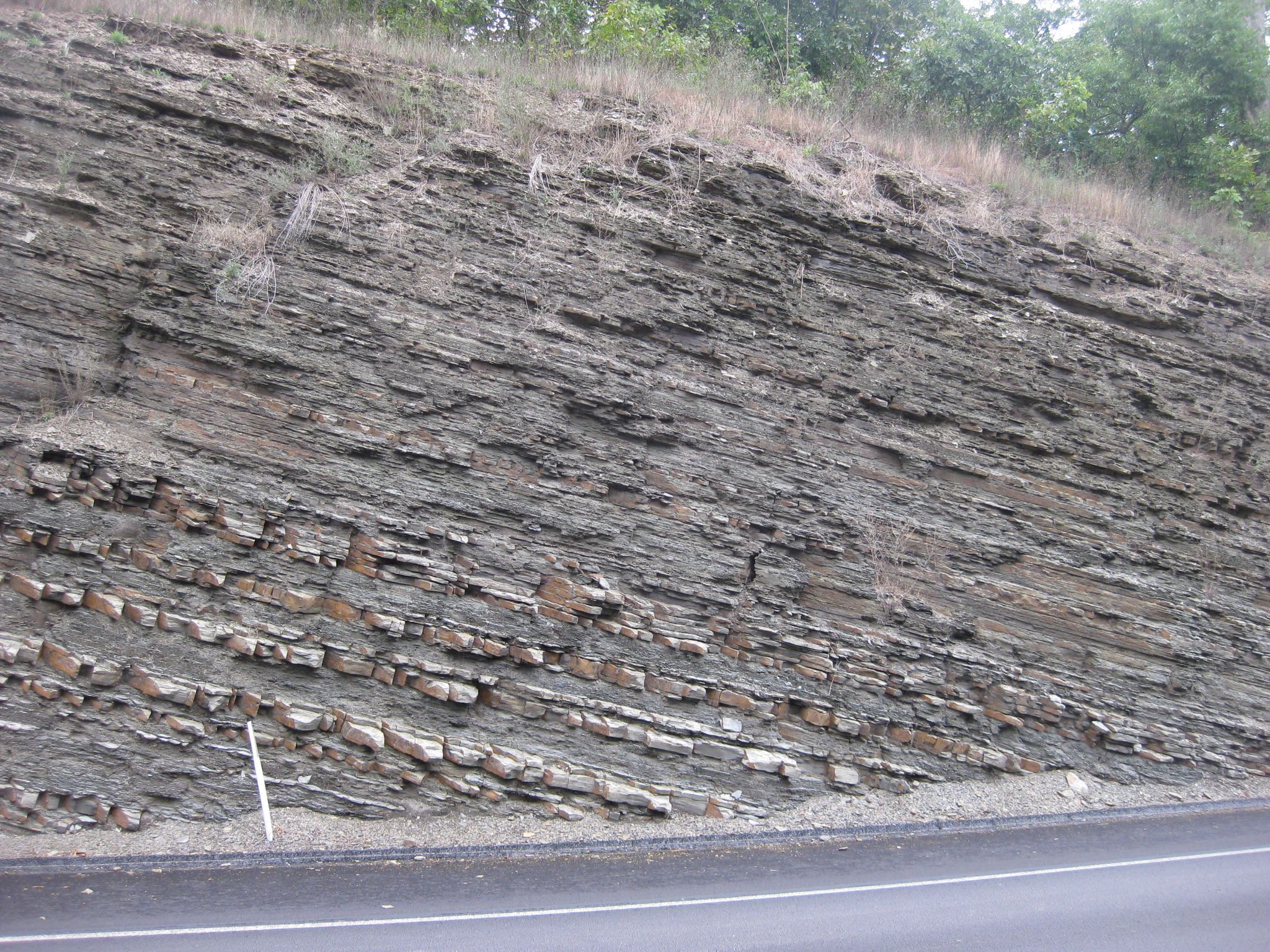
Figure 5.24 – Outcrop of Devonian Brallier Formation on the north side of the Pennsylvania Turnpike, central Bedford County, near Mile Marker 138 in Pennsylvania. Sandstone beds near the bottom of the photo are possible turbidites. Image credit: Wikimedia user Jstuby, CC0 Public Domain, photo taken August 2011. Sketch Area: - Figure 5.25 is a roadside outcrop of the Hampshire Formation in Pennsylvania, composed of sandstone and fine-grained siltstone. Provide a sketch of this outcrop.
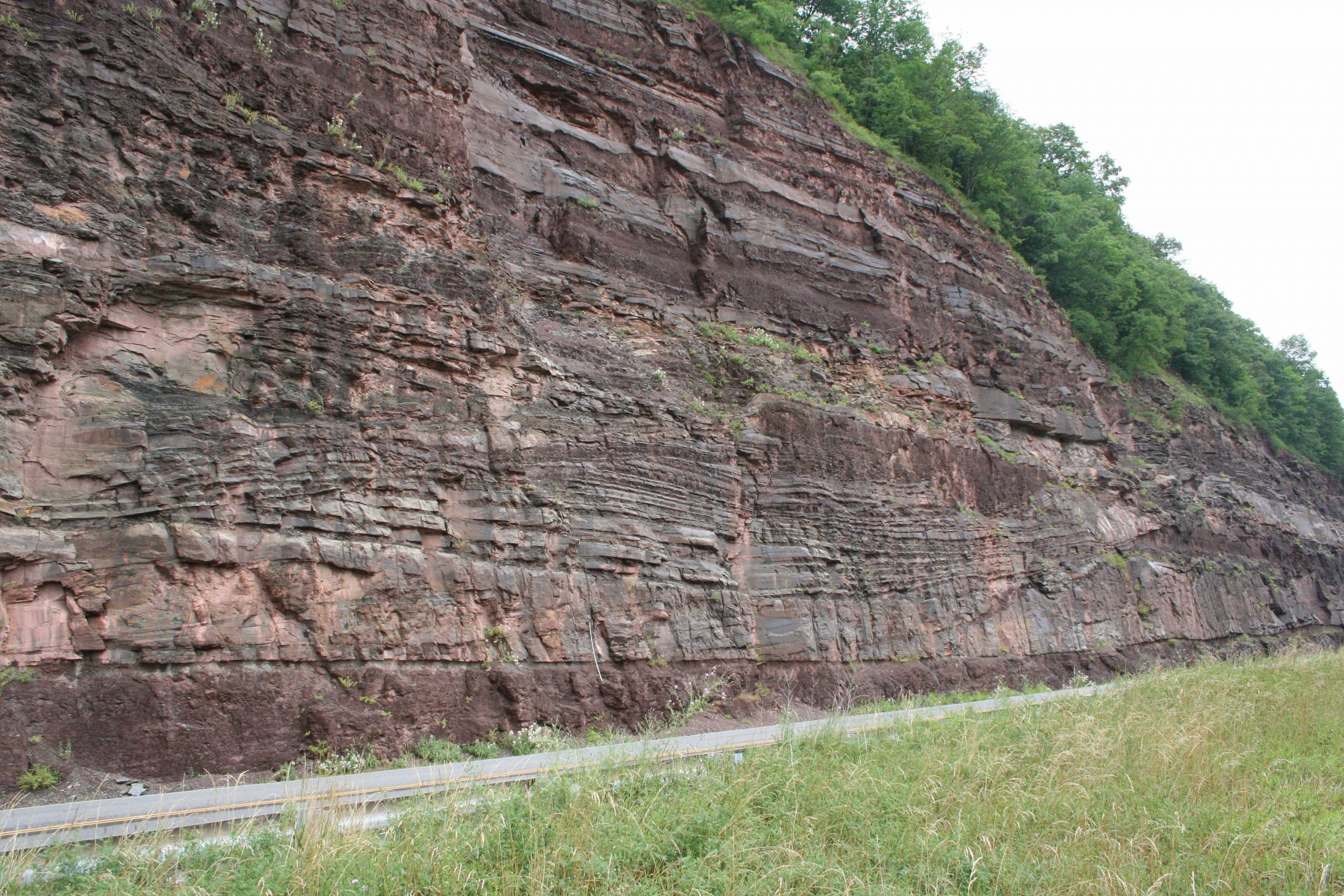
Figure 5.25 – Point bar deposits in the Hampshire Formation near North Bend, Pennsylvania. Image credit: Wikimedia user Rygel, M. C., CC BY-SA. Sketch Area: - What sedimentary structure is shown in Figure 5.25, and can you tell in which direction sediment was being transported?
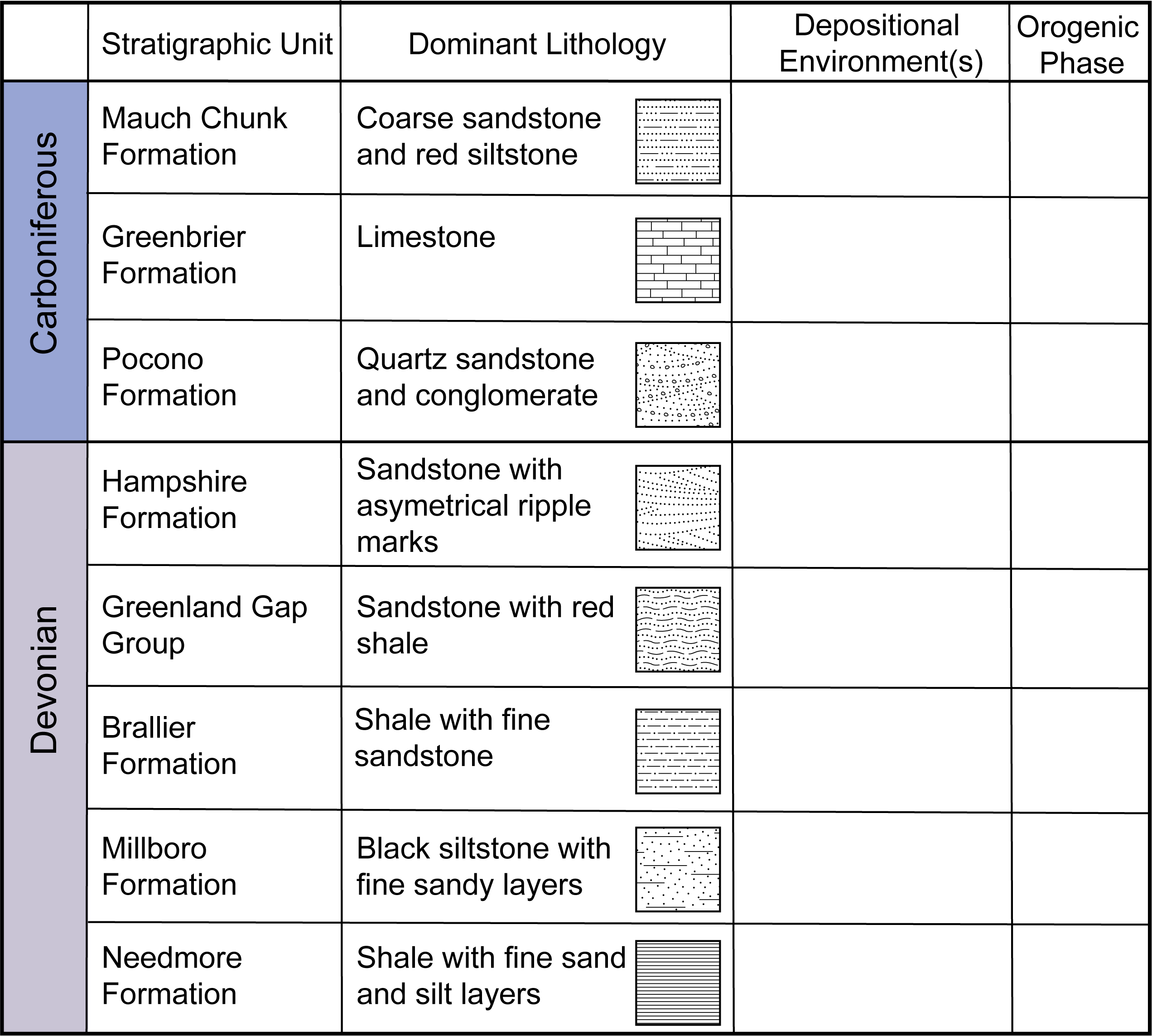
- Figure 5.26 below contains the sequence of sedimentary rocks associated with the Catskill clastic wedge. Based on the rock descriptions, identify the depositional environment for each stratigraphic unit and which orogenic phase it represents.
- Figure 5.24 is a roadside outcrop of the Brallier Formation in Pennsylvania, composed of shale and fine sandstone layers. Provide a sketch of this outcrop and identify the layers of sandstone vs. the layers of shale.
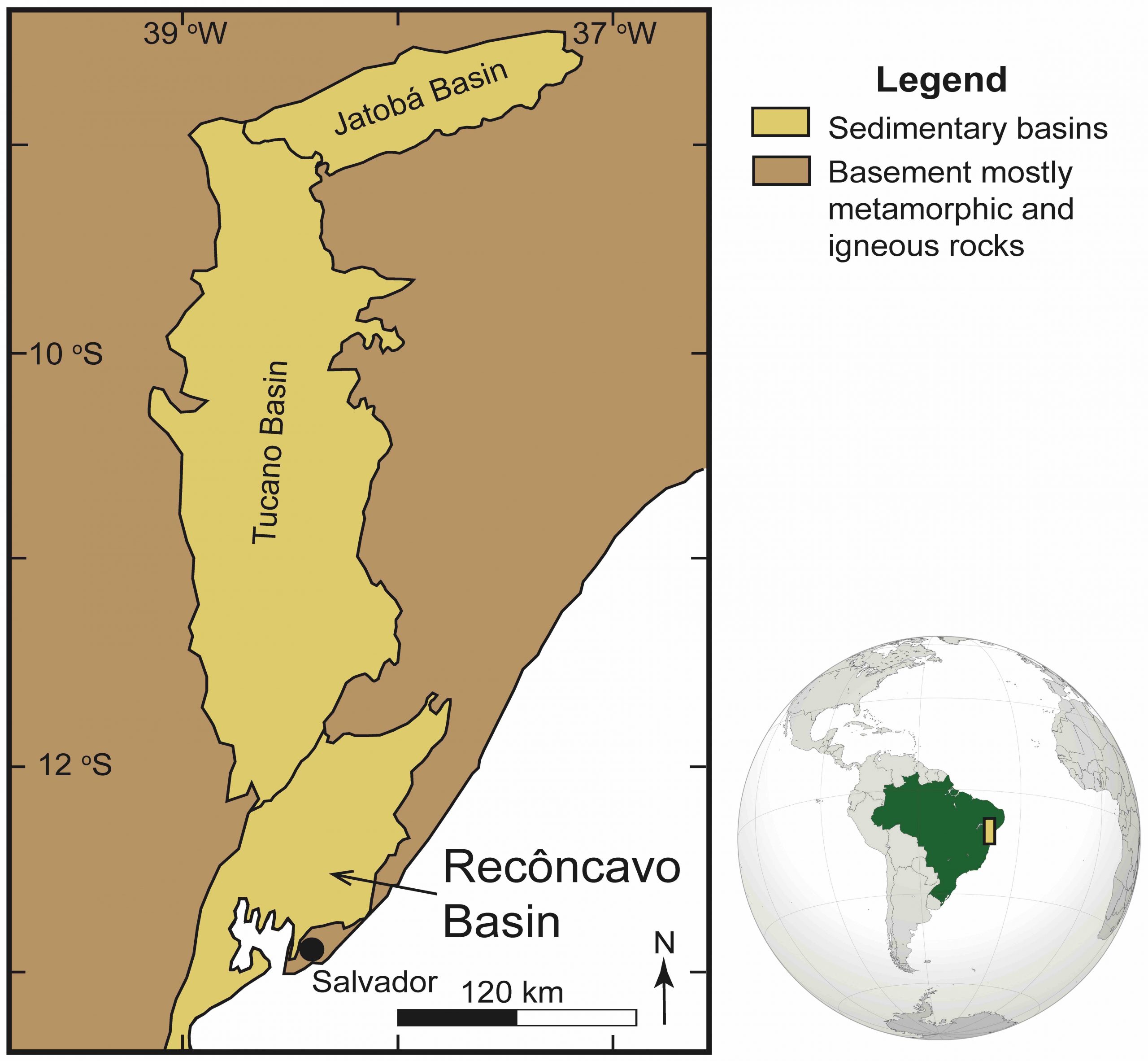
Another dynamic aspect of plate tectonics is continental rifting, a process in which a continental mass splits apart and two separate new landmasses form and drift away from each other. After the last orogeny in the Appalachian mountains, Pangea broke apart into our current continent configuration through continental rifting processes. The Recôncavo basin in Brazil near the city of Salvador (Figure 5.27) is the southernmost basin in northeastern Brazil created by continental rifting of South America and Africa. This rifting process is well recorded in the eastern Brazilian margin and shows different stages of this process:
- Before rifting begins, continental processes such as fluvial, eolian, and lacustrine deposition dominate the sediment deposition.
- Then as the rifting begins, igneous activity also begins. In continental rifts, this is usually bimodal (rhyolite and basalt) volcanism. Rifting also causes normal faulting of the continent forming grabens and half grabens resulting in lacustrine (lake) deposits. In some areas, very high-energy processes dominate. As the continent starts to split apart, the ocean water will flood the depression caused by the faulting creating shallow-water seas, which sometimes host various shallow marine species.
- As the shallow seas and lakes are evaporated, massive salt and anhydrite (evaporites) deposits are formed.
- Rifting completely separates the continent into two new landmasses, which start drifting apart and are marked by a “passive margin system.” Tectonic activity is no longer present, and the sediments are increasingly deeper marine.
Exercise 5.11 – Continental Rifting in a Sedimentary Record
Stratigraphic Evidence of Continental Rifting
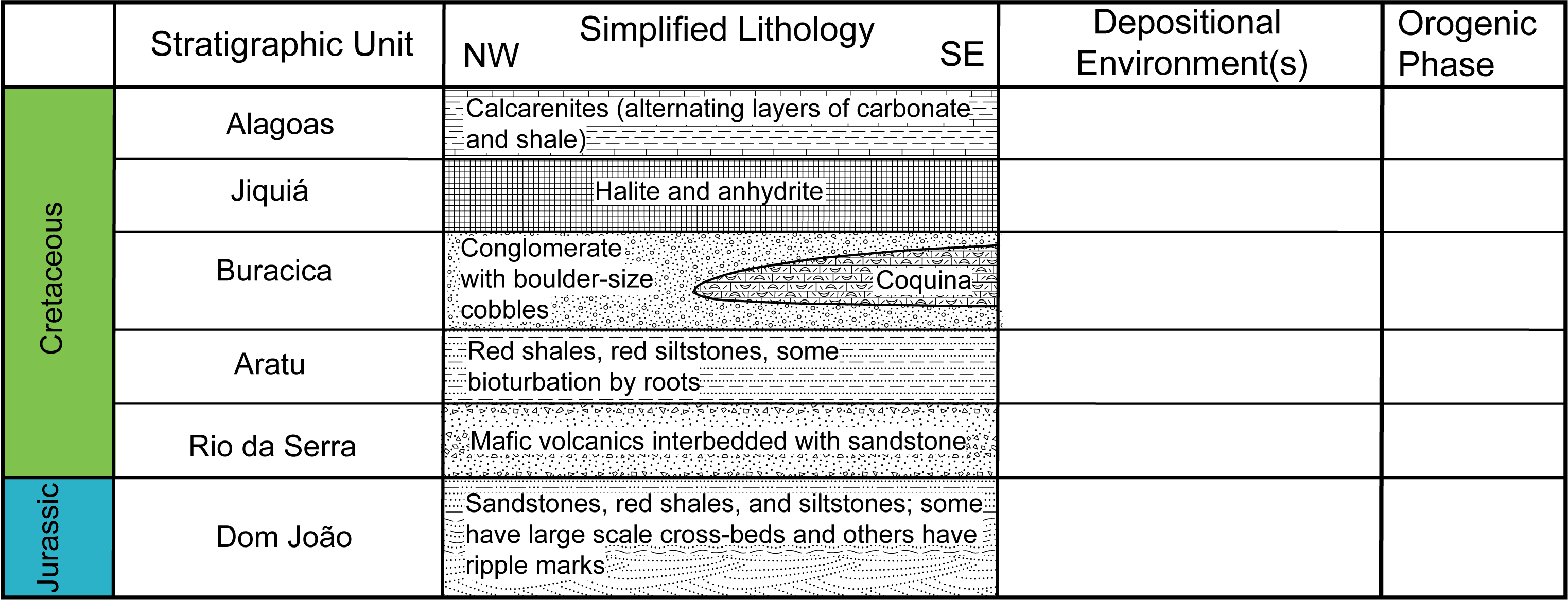
- Determine the depositional environments for the different lithologies in the northeastern Brazilian Recôncavo Basin’s stratigraphic column in Figure 5.28 below.
- Identify the 4 stages of rifting (described above Figure 5.28) and mark them 1, 2, 3, and 4 in the right-most column in Figure 5.28. Mark your boundaries between the stages by drawing a thick line at the top of the formation that ends each stage.

Figure 5.28 – Stratigraphy of the Brazilian Recôncavo Basin with simplified lithology. Image credit: Carlos Andrade and Virginia Sisson CC BY-NC-SA. - Critical Thinking: What will the sedimentary environment be in this part of Brazil after rifting has stopped?
- Critical Thinking: Today, the Atlantic Ocean marks the rift boundary between Brazil and Africa. At what stage did the rifting stop in the Recôncavo Basin? Why?
Outcrop Interpretations
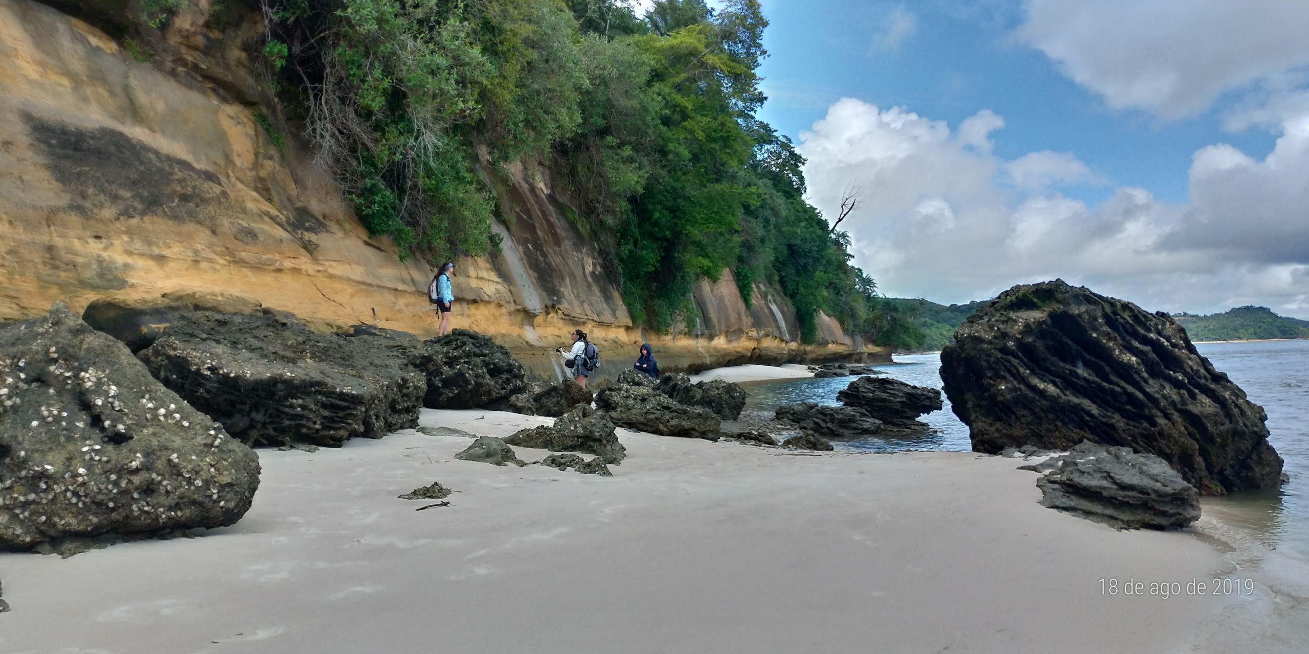
The following questions refer to Figure 5.29.
- What sedimentary environment do you find oysters in?
- Why is the rock in Figure 5.29 black?
- What is the sedimentary environment of the overlying buff-colored layers?
- How does this change in sedimentary environments fit with the tectonic setting of the Recôncavo Basin?
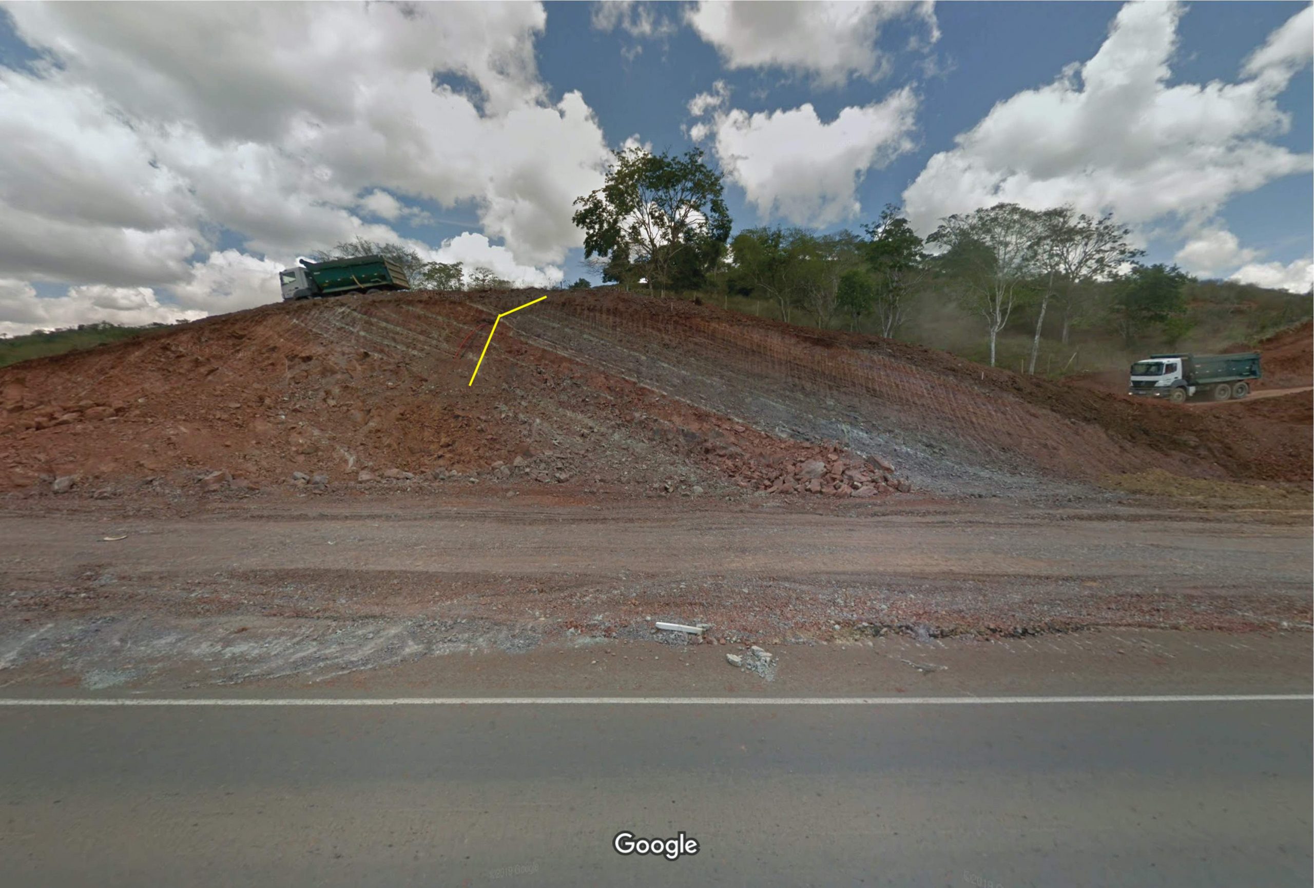
Figure 5.30 – Dom João Formation along BR 101, about 14 km southwest of Algoinhas, Brazil. Two processes cause the red color; one is intense tropical weathering creating red soil (the left side of the outcrop is almost completely converted into red soil as is a layer at the top of the outcrop), and two, hematite oxidation during deposition of these sandstones and shales. A fault offsets the bedding in this outcrop along the yellow line. Image credit: Google Street View. - What type of fault is present in Figure 5.30? It may help you to draw arrows on either side of the fault showing the sense of motion. ____________________
- What is the age of the fault (remember to look at the stratigraphic column for the age of the formation)? ____________________
- Is this fault related to continental rifting? How does this help you determine the depositional environment?
Additional Information
Exercise Contributions
Daniel Hauptvogel, Virginia Sisson, Carlos Andrade, Joshua Flores, Melissa Hansen
References
Krumbein, W.C., and Sloss, 1963, Stratigraphy and Sedimentation (2nd edition), W.H. Freeman and Co., 660 p.
Magnavita, L., Da Silva, R.R., and Sanches, C.P., 2005, Field trip guide of the Recôncavo basin, NE Brazil, April 2005, Boletim de Geociencias – Petrobras, 13(2), 301-333.
Miller, K.G., Kominz, M.A., Browning, J.V., Wright, J.D., Mountain, G.S., Katz, M.E., Sugarman, P.E., Cramer, B.S., Christie-Blick, N., and Pekar, S.F., 2005, The Phanerozoic Record of Global Sea-Level Change, Science, 310, 1293-1298. doi: 10.1126/science.1116412
Moore, G.F., Park, J.-O., Bangs, N.L., Gulick, S.P., Tobin, H.J., Nakamura, Y., Sato, S., Tsuji, T., Yoro, T., Tanaka, H., Uraki, S., Kido, Y., Sanada, Y., Kuramoto, S., and Taira, A., 2009. Structural and seismic stratigraphic framework of the NanTroSEIZE Stage 1 transect. In Kinoshita, M., Tobin, H., Ashi, J., Kimura, G., Lallemant, S., Screaton, E.J., Curewitz, D., Masago, H., Moe, K.T., and the Expedition 314/315/316 Scientists, Proc. IODP, 314/315/316: Washington, DC (Integrated Ocean Drilling Program Management International, Inc.). doi:10.2204/iodp.proc.314315316.102.2009
Mull, C.G., Houseknecht, D.W., and Bird, K.J., 2003, Revised Cretaceous and Tertiary Stratigraphic Nomenclature in the Colville Basin, Northern Alaska: U.S. Geological Survey Professional Paper 1673, 51 p.
Payne, T.G., 1951, Geology of the Arctic slope of Alaska: U.S. Geological Survey Oil and Gas Investigations Map 126, 3 sheets, scale 1:1,000,000.
Picard, M.D., 1971, Classification of fine-grained sedimentary rocks, Journal of Sedimentary Petrology, 41, 179-195. https://doi.org/10.1306/74D7221B-2B21-11D7-8648000102C1865D
Vail, P.R., Mitchum, R.M., and Thompson, S., 1977, Seismic stratigraphy and global changes of sea level, part 3: Relative changes of sea level from coastal onlap, in C.E. Clayton, ed., Seismic stratigraphy – applications to hydrocarbon exploration: Tulsa, Oklahoma, American Association of Petroleum Geologists Memoir 26, 63–81.
Vérard, C., Hochard, C., Baumgartner, P.O., and Stampfli, G.M., 2015, 3D paleogeographic reconstructions of the Phanerozoic versus sea-level and Sr-ratio variations, Journal of Palaeogeography, 4, 64-84. doi:10.3724/SP.J.1261.2015.00068
Google Earth Locations

a branch of geology that focuses on the study of rock layers and layering. It is can cover both sedimentary and layered volcanic rocks. Stratigraphy has two related subfields: lithostratigraphy and biostratigraphy
another term for reflection coefficient or how much energy is reflected by the stratigraphic units
a fundamental rock unit based on similar characteristics in lithology, including characteristics as color, mineralogy, and grain size. Formations may represent deposition over short or long time intervals, may be composed of materials from several sources, and may include breaks in deposition. Formations are named after geographic features where they were first studied.
a seismic reflector may represent a change in lithology, a fault, or an unconformity
a set of characteristics with similar seismic reflections including bedforms, their geometry, lateral continuity, amplitude, frequency, and interval velocity
composed of fragments or clasts, of geologic detritus including both minerals and rocks
the amount of void space in a rock
the ability for fluids (including gas) to flow through rocks
a graph that depicts the ratios of the three variables as positions in an equilateral triangle
a geologic period that spans 50.6 million years from the end of the Permian Period 251.9 Ma, to the beginning of the Jurassic Period 201.3 Ma. This is the first and shortest period of the Mesozoic Era
a geologic period that spanned 56 million years from the end of the Triassic Period 201.3 Ma to the beginning of the Cretaceous Period 145 Ma. This constitutes the middle period of the Mesozoic Era, also known as the Age of Reptiles
an extensive area of predominantly iron- and magnesium-rich (mafic) rock that form by processes other than normal seafloor spreading; they are the dominant form of near-surface magmatism on the terrestrial planets and moons of our solar system
a sub-discipline of stratigraphy focuses on strata or rock layers
for sedimentary rocks, it is a body of rock with specified characteristics such as type of sediment
parallel strata that have a similar geologic history and were deposited in succession without interruption
a geologic event during which sea level rises relative to the land and the shoreline moves toward higher ground, resulting in flooding
a geological process occurring when areas of previously submerged seafloor are then exposed above sea level
Areas of land that are covered by a sedimentary basin and are now below sea level. A marine transgression is a geological process occurring when areas of land are submerged below sea level. The opposite event, marine regression, occurs when the sea becomes exposed land (transgressive). Synonym: onlap
Areas of submerged seafloor being exposed above the sea level. A marine regression is a geological process occurring when areas of submerged seafloor are exposed above the sea level. The opposite event, marine transgression, occurs when flooding from the sea covers previously-exposed land (transgressive).
area of geology that deals with the distribution and movement of groundwater in the soil and rocks of the Earth's crust
a body of rock and/or sediment that holds groundwater
the beach between the foreshore and coastline. The backshore is typically dry and does not have vegetation and often characterized by berms or dunes. The backshore is only exposed to waves under extreme events with high tide and storm surge
there are two types of dunes: subaerial and subaqueous. Most only know about the subaerial dunes from trips to the beach and/or a desert. They are made of wind-blown sand and typically are vegetated. Subaqueous dunes are also known as sandwaves.
this is the zone between low-tide line and high-tide line, also called the beach face. It is typically wet from the tides and waves and can be destroyed by storm surge.
area of relatively shallow water in a coastal environment, separated from the open marine conditions by a natural barrier (a sand spit, a barrier island or a coral reef), but with an access to the sea
in coastal areas, these are low-lying and often inundated by tidal waters. They tend to be heavily vegetated and low-energy sedimentary environments.
this zone extends from the low-tide line to beyond where waves influence the sedimentation (sometimes called the breaker zone).
caused by waves that rush over a natural or artificial coastal barrier. This term can also be used for the sand deposit on the leeside of the barrier. These typically form during storm events.
the branch of stratigraphy that uses fossils to determine relative age and correlate successions of sedimentary rocks
gamma (γ) rays come from the radioactive decay of naturally occurring radionuclides
a rock property which represents how strongly it opposes the flow of electric current
of the amount of electrical current a rock can carry or its ability to carry a current
a branch of stratigraphy in which stratigraphic divisions are made on the basis of changes in magnetic signals
these sedimentary layers are timelines that represent a moment in geological time
a geological period from about 145 to 66 Ma. It is the third and final period of the Mesozoic Era, as well as the longest. The name is derived from the Latin creta, chalk
the current geologic eon in the geologic time scale. This has the abundant animal and plant life. It covers 541 million years to the present, and it began with the Cambrian Period
a basin formed between two adjacent strike-slip faults in a region where subsidence generates accommodation space for the deposition of sediments
a mountain building period from 550 to 440 million years ago
a mountain building period from 420 to 380 Ma
a mountain building period from 350 to 250 Ma
the principle that Earth's crust is floating on its mantle
structural basin that develops adjacent and parallel to a mountain belt formed from the mass created by crustal thickening that causes the lithosphere to bend creating accommodation space
graben and horst refer to regions between normal faults and are either higher (horst) or lower (graben) than the area beyond the faults
