
Chapter 11 – Interpreting Maps
This book contains exercises for a physical geology lab class. It is under development, with a full 1st edition release planned for Fall 2024.
The goals of this chapter are to:
- Evaluate latitude and longitude
- Determine compass directions
- Understand and construct topographic maps and profiles
An important part of geologic field work is noting the precise locations of samples, outcrops, geologic features, etc. If you or other scientists cannot return to find your exact study site, then the science cannot be reproduced. Part of being a scientist is creating data, an experiment, etc. that is reproducible.
In Chapter 1 you briefly explored the different coordinate systems for maps: Degree Minutes Seconds (DMS) and Decimal Degrees (DD). Which system you use may depend on how you keep track of your study sites. That means it’s important to not only understand different coordinate systems but also be able to convert coordinates between systems.
DMS divides the roughly spherical planet Earth into 360 slices that are each 1°, each degree is broken down into 60 smaller slices called minutes, and each minute is broken into 60 smaller slices called seconds. DD converts the three numbers used to define a coordinate with DMS into a single number using a simple calculation. Below is a diagram showing how to convert a single coordinate back and forth between DMS and DD.
Exercise 11.1 – Converting Geographic Coordinates
Figure 11.1 shows you how to convert a single coordinate back and forth between DMS and DD.

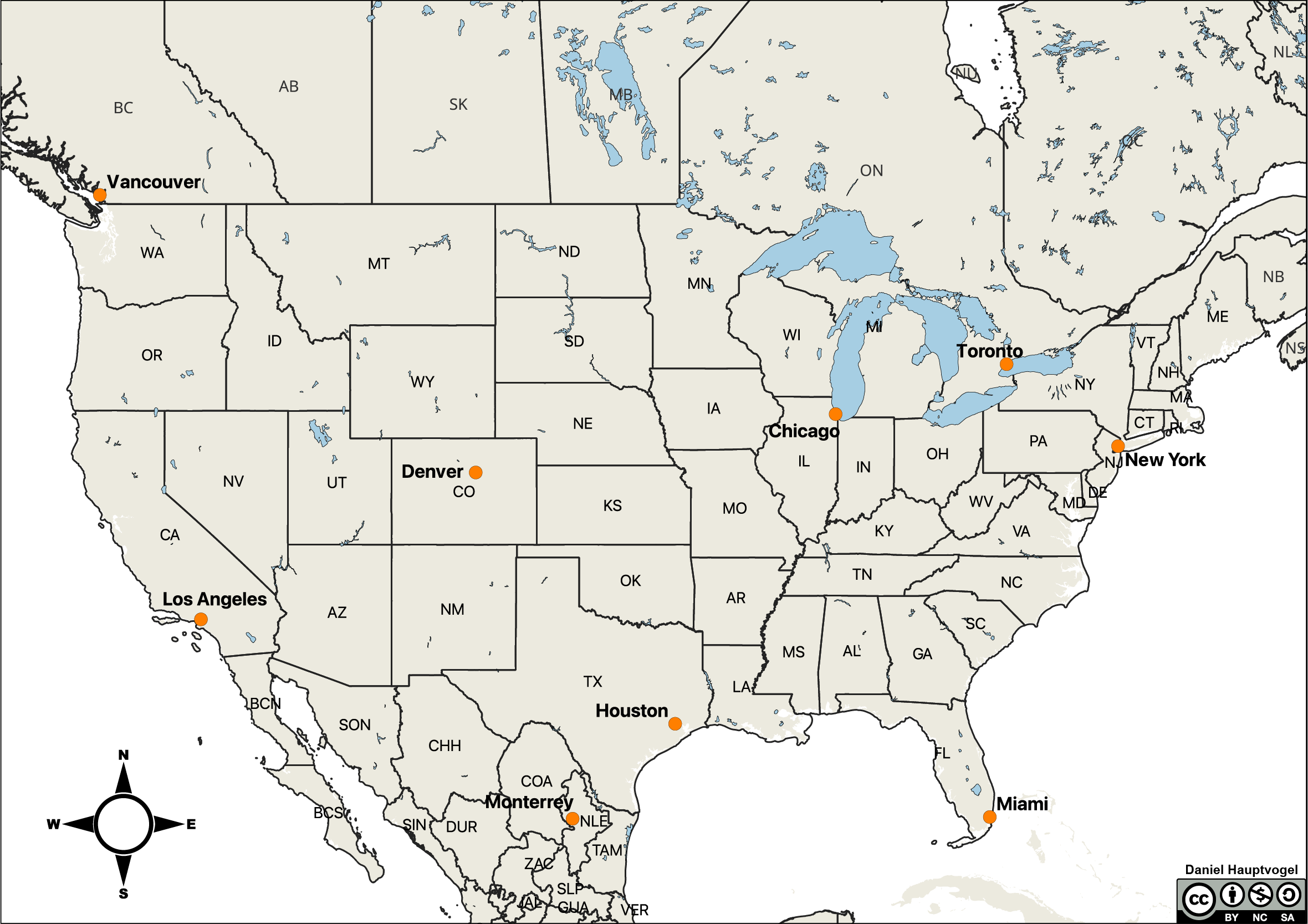
- Table 11.1 contains geographic coordinates for some cities, as shown in Figure 11.2. One of the coordinate systems is given for each city. Using Figure 11.1, convert coordinates to either DMS or DD. Denver, CO has been done for you.
Table 11.1 – U.S. cities and their geographic coordinates Degrees Minutes Seconds (DMS) Decimal Degrees (DD) Denver, CO 39° 44′ 21″ N, 104° 59′ 25″ W 39.7392 N, 104.9903 W New York, NY 40° 42’ 46” N, 74° 00’ 22” W Los Angeles, CA 34.0549 N, 118.2426 W Monterrey, Mexico 25.6866 N, 100.3161 W Chicago, IL 41° 51’ 55” N, 87° 37′, 40” W Houston, TX 29° 45’ 46” N, 95° 22’ 59” W Toronto, Canada 43.6532 N, 79.3832 W - Which coordinate system do you think is better and why?
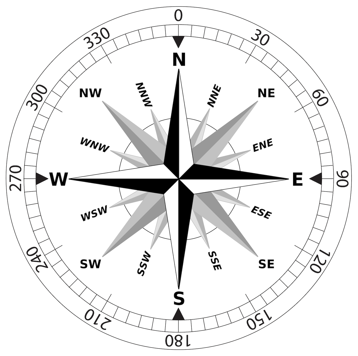
An important part of reading maps is understanding how to use a compass. As a geologist, you may want to know the direction a rock unit is dipping, the direction from one mountain peak to another, or the direction a paleo-river used to flow. There are two forms of direction that you should be familiar with: the cardinal directions and azimuth system (Table 11.2 and Figure 11.3).
Exercise 11.2 – Compass Directions
| Cardinal | Azimuth |
| N | 0° |
| NNE | 22.5° |
| NE | 45° |
| ENE | 67.5° |
| E | 90° |
| ESE | 112.5° |
| SE | 135° |
| SSE | 157.5° |
| S | 180° |
| SSW | 202.5° |
| SW | 225° |
| WSW | 247.5° |
| W | 270° |
| WNW | 292.5° |
| NW | 315° |
| NNW | 337.5° |
Now you can practice your compass skills.
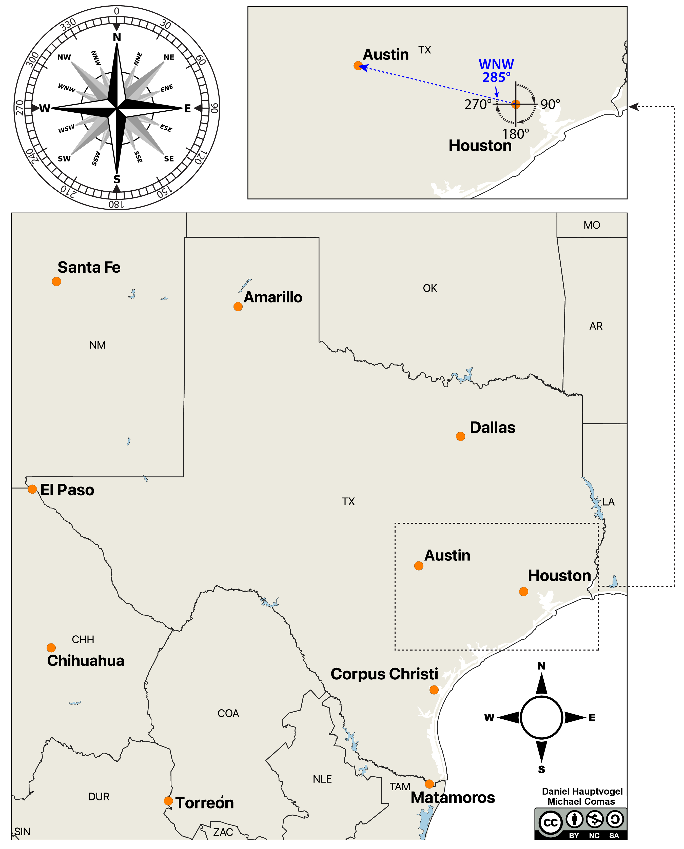
- Without using a protractor, what is the compass direction (NW, WNW, E, SE, etc.) between the following cities in Figure 11.4 (Houston to Austin example completed for you)?
- Houston to Austin: WNW
- El Paso to Santa Fe: ____________________
- Santa Fe to Dallas: ____________________
- Dallas to Torreon: ____________________
- Torreon to Matamoros: ____________________
Follow the steps below to find the direction (azimuth) between cities in Texas in Figure 11.4. An example has been provided along with the steps for determining the azimuth from Houston to Austin.
- Use a straight edge to draw a line between your two points
- Place the cross of the protractor on your starting point and orient the 90° mark on the protractor towards the north if the second point is to the north or towards the south if the second point is to the south.
- Determine how many degrees away from 0 your line is pointing.
- Now, use a protractor and find the azimuth directions for the cities below (Houston to Austin example completed for you).
- Houston to Austin: 285°
- Matamoros to Austin: ____________________
- Austin to Chihuahua: ____________________
- Chihuahua to Amarillo: ____________________
- Amarillo to Houston: ____________________
Maps are scaled-down versions of the areas they represent. The word “scale” refers to the amount of reduction the map represents. All maps include at least one type of map scale to indicate the relationship between the area on the map and the area of the region it represents in reality. Map scales are provided so that a map reader can determine exactly how much distance is actually represented on their map, or to measure the distance between two points on a map, or even to calculate the gradient (slope) of a hill, valley, or river.
The two commonly used map scales on a topographic map are the bar scale and the fractional scale (also known as the ratio scale). A common ratio scale used in topographic maps is 1:24,000, which means that 1 unit of measurement on the map is 24,000 units in reality. The unit does not matter because the principle works the same for all units; it could be inches, feet, centimeters, etc.
Exercise 11.3 – Map Scales
You can use your knowledge of scales to estimate distances on maps.
- On a map with a scale of 1:12,000, how long is a stream (in feet) that measures 1 inch on the map? ____________________
- On a map with a scale of 1:40,000, how long is a road (in meters) that measures 5 cm on the map? ____________________
- Your instructor will provide you with two maps of the Galveston, TX region at different scales. One was published in 1983, the other in 2022. What are the scales of each map?
- Look closely at both maps. What information is given on the 2022 map that isn’t on the 1983 map, and vice versa?
- On the northeast side of the 2022 map, measure the channel width between Galveston Island (Fort Point) and Point Bolivar. How wide is the channel on the map (cm) and in reality (m and mi)?
- Do the same measurements using the map from 1983.
- Which map is better for determining this distance? Why?
- These maps were published 39 years apart. Can you think of any reason why this may have affected your measurements?
- Do you think it is important that maps be updated often? Should certain geographic regions be re-mapped more often than others? Why?
- Which map would be best to use to show the projected approach of a hurricane toward the Texas coast? Why?
- Which map would best display detailed hurricane evacuation routes off of Galveston Island. Why?
- Which map should a cruise ship captain use to help guide him into the port at Galveston? Why?
Topographic maps show the topography of the landscape, including hills, mountains, valleys, rivers, etc. These maps contain contour lines, which are lines of equal elevation. That means everywhere along that line will have the same elevation.
Elevations for major contour lines are typically marked on the line. To avoid clutter, not every contour is labeled. The elevation of an unlabeled contour line can be determined by knowing the contour interval and looking at adjacent contour lines. The elevation of a point located in between two contour lines can be estimated by interpolating between the lines. If a point is halfway between two contour lines, it will be about halfway between the elevations of those two contour lines.
In the US, topographic maps have elevation marked in feet or meters above mean (average) sea level. International maps and maps of elevation of the ocean floor (bathymetry) are usually marked in meters.
Exercise 11.4 – Contour Lines and Topographic Maps
Capulin Volcano in New Mexico (Figure 11.5) is a volcanic cinder cone that is about 60,000 years old. Figure 11.6 is a map view and topographic map of the volcano.


- What pattern do you notice in the contour lines that represent the volcano?
- A contour interval is the elevation difference between contour lines. Some lines are bold; these are major contours and are marked at regular intervals. On this map, the major contours are 50 m apart. What is the contour interval of this map? ____________________
- What is the elevation of the highest point of Capulin Volcano? ____________________
- How deep is the crater of the volcano? ____________________
- If you either walk or drive from the visitor’s center to the scenic overlook, how much would your elevation have changed? ____________________
- Topographic maps also give you a sense of the slope of the landscape. Examine the eastern and western sides of Capulin Volcano. Which side is steeper, and which is shallower? What does the spacing of the contour lines tell you about the slope?
- Construct a topographic profile of this area in Google Earth. Your instructor will help you.
On a contour line on a map, elevations on one side of a line will be lower elevations, and elevations on the other side of a line will be higher elevations. So, your contour line can help you determine which way the topography goes up and down hills, valleys, and rivers.
The rules inherent in topographic maps are pretty simple: contours represent lines of equal elevation, contours always close (except on the edge of a map), contours never cross although they may become very close on steep terrain or cliffs, closely spaced contours represent steepness, and the geometry of contours changes in predictable ways between valleys and ridges. The latter is called the Rule of Vs, where:
- contours V up-gradient (upstream) in valleys, and
- down gradient on adjacent ridges.
Exercise 11.5 – Exploring Rules of Contour Lines
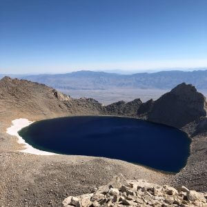
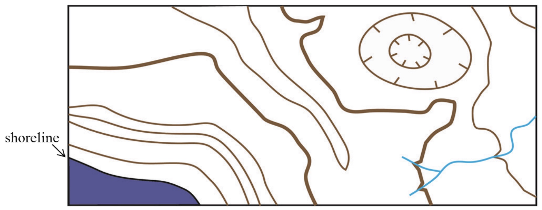
Below is an image from the high peaks of the Sierra Nevada and a simplified topographic map of this area. Use these to discover some other rules of topographic maps. Examine the photo and map in Figures 11.7 and 11.8.
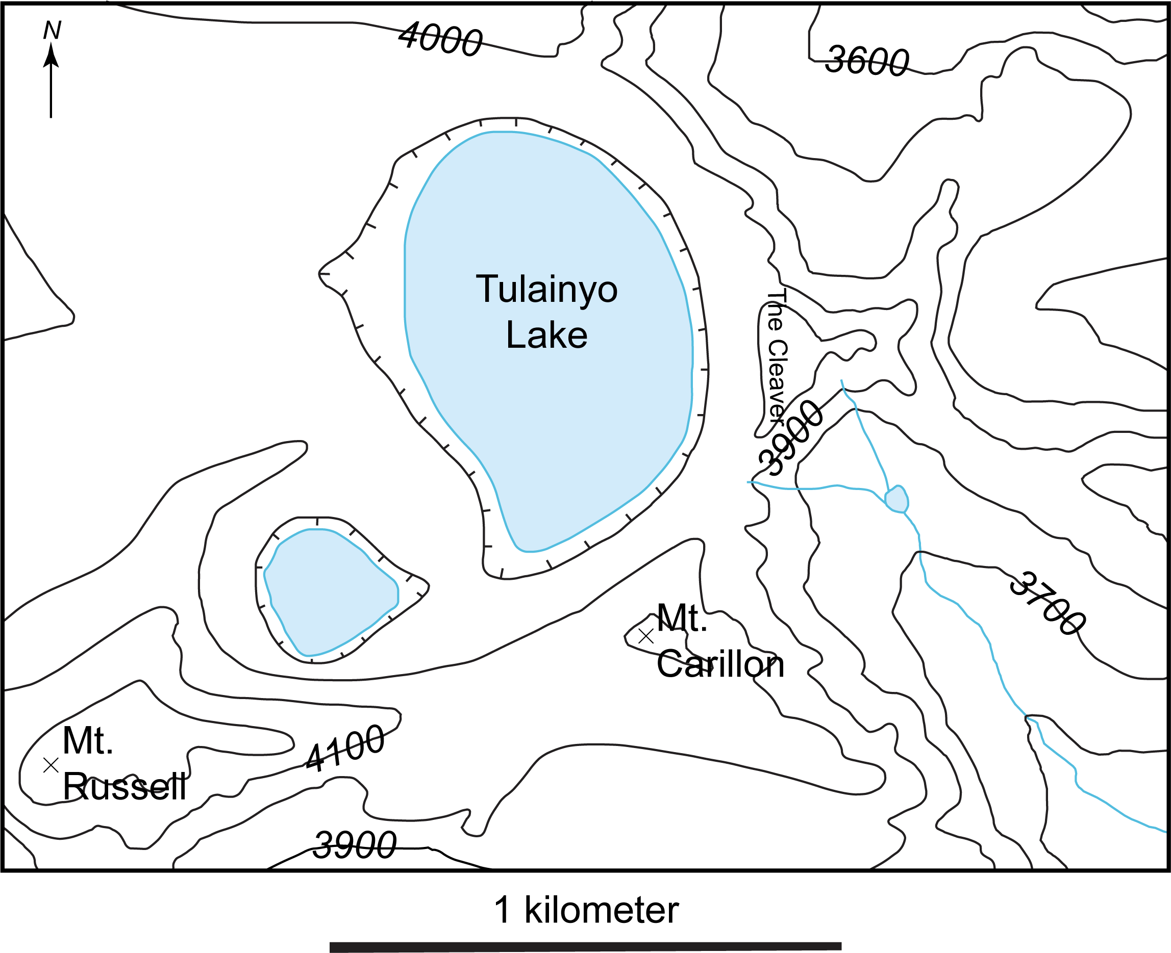
- Look at the stream in the southeastern side of the map. What happens to contour lines when they cross a stream? Your instructor may also provide you with block models to illustrate this rule.
- Tulainyo Lake and an unnamed lake in this map have little hatch marks around them. What do these mean?
- Do the contour lines ever cross each other? Why or why not?
- Where are the lowest and highest elevations in this map? ____________________
- What do the cross marks indicate for Mount Russell and Mount Carillon?
- Critical thinking: The contour interval is 100 m (328 ft). Do you think this is adequate to show the topography in this region (look at a photo of the area). What contour interval would you prefer and why?
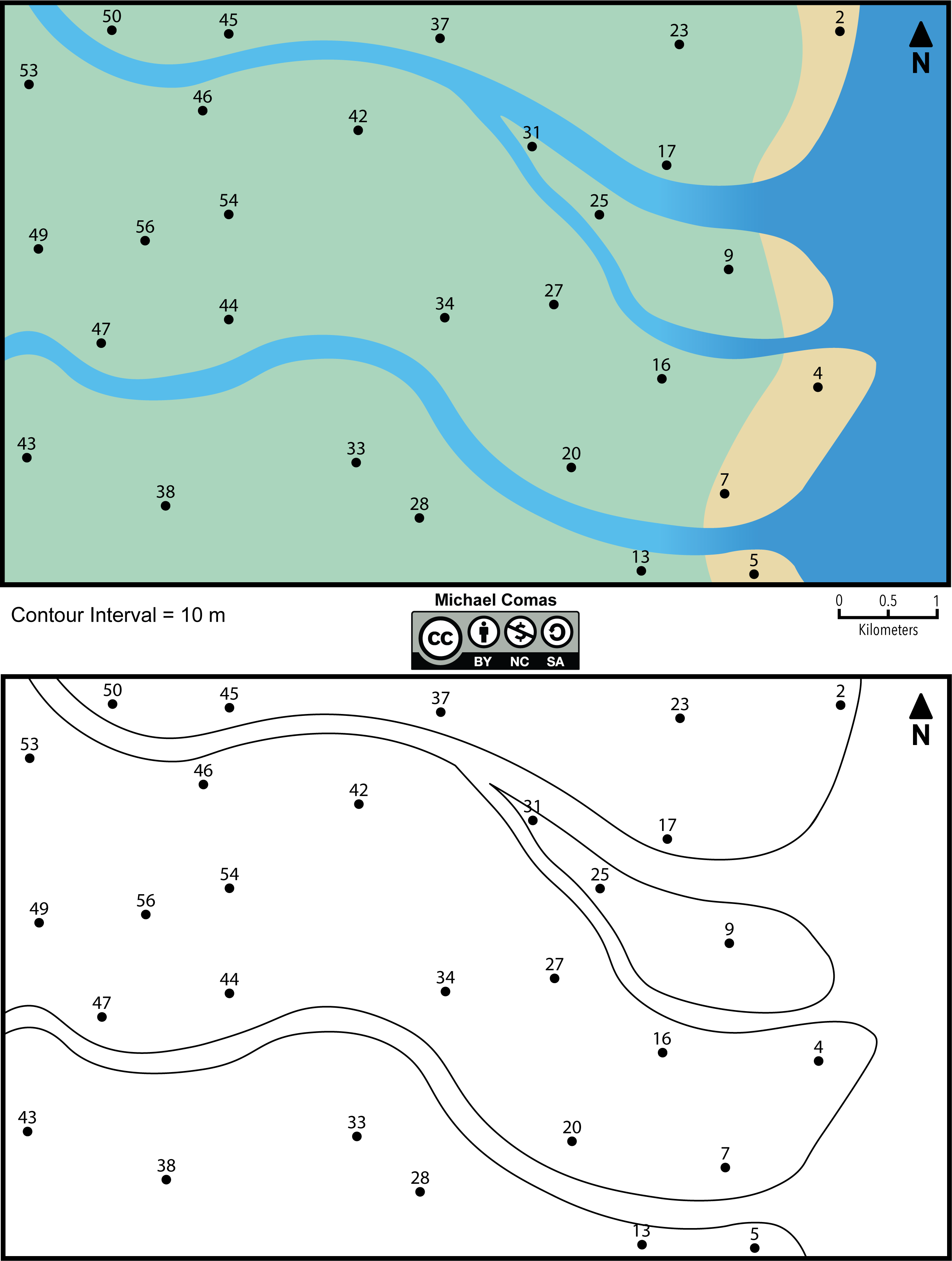
- Build your own contour map. Use the elevation data to make your own contour map from the data in Figure 11.9. The contour interval will be 10 m. The zero-contour interval is at sea level; so, you don’t need to draw that one! You may have to interpolate and extrapolate the data as there are very few data points that are 10 m intervals. Remember how the contour intervals should look around the small streams and rivers. Draw your contour lines so that they are continuous: they will either continue to the edge of the map or form an enclosed circle.
To get a good sense of the landscape, geologists construct topographic profiles (Figure 11.10). To do this, use these five steps:
- Place a strip of paper along the line of the profile you are making (W-E) and label the starting and ending points (Figure 11.10).
- Mark the paper where it comes into contact with any contour lines and label each mark with the corresponding elevation.
- Choose your vertical scale and prepare a sheet of graph paper by labeling the vertical axis according to the scale you have chosen. It is typically best to choose a range of elevations that encompass your profile elevations (for example, if the Volcano’s elevations ranged from 223-339 meters, it may be best to choose a scale from 200-350 meters).
- Place your strip of paper with the labeled marks (from Step 2) at the bottom of the vertical scale and use the elevation data to plot points on your graph.
- Trace the points from one side of the profile to the other.
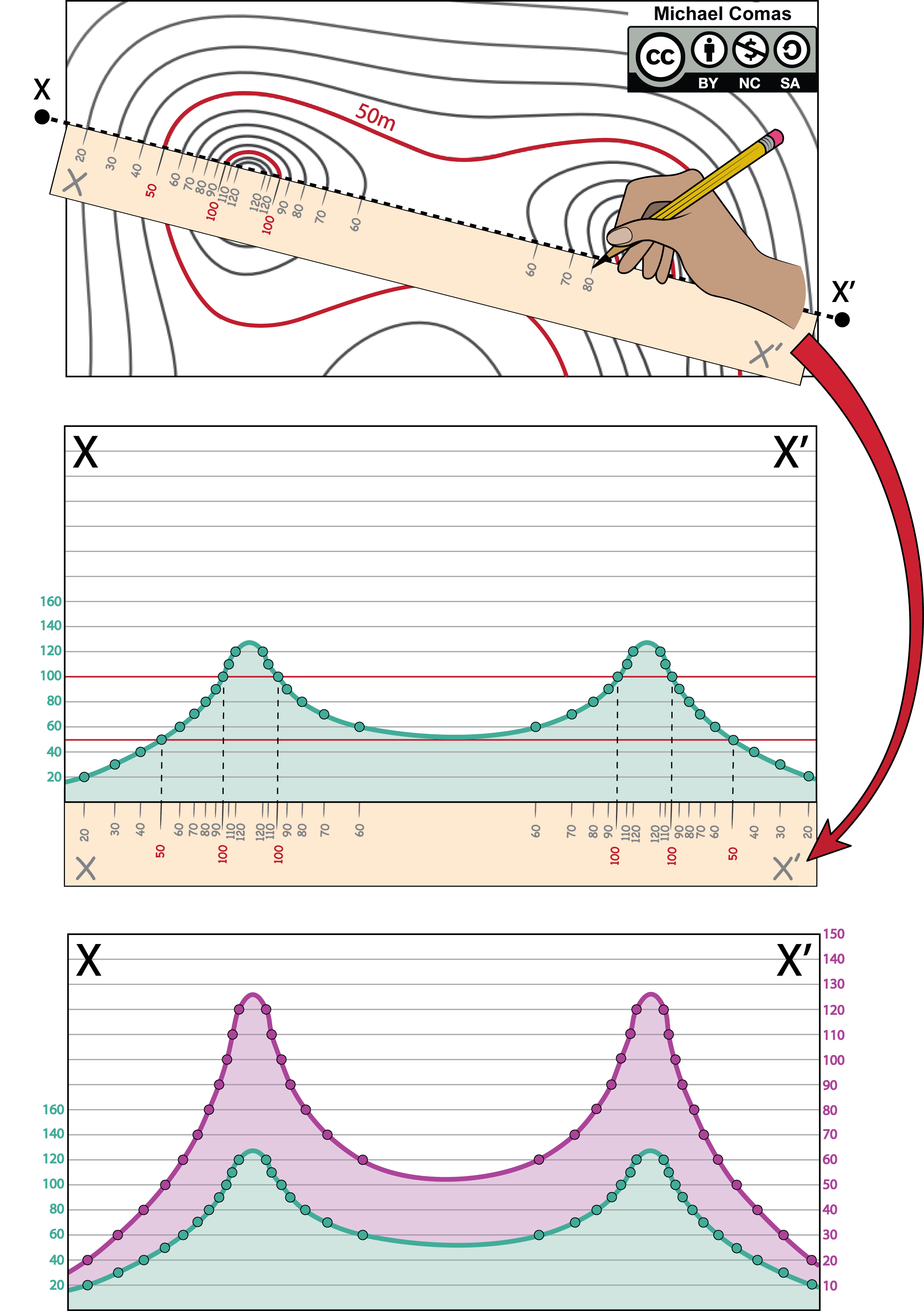
Figure 11.10 – How to construct a topographic profile. Image credit: Michael Comas, CC BY-NC-SA.
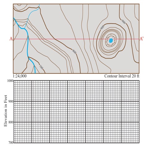
Exercise 11.6 – Constructing a Topographic Profile
Make a topographic profile for Figure 11.11.
Hands on exercises are fun. So, welcome to the exciting world of augmented reality (AR)! You may have used this AR in exercise 1.x with the augmented reality sandbox. This innovative project combines the physicality of a sandbox with the virtual elements, giving you a unique and interactive experience. This is a system that combines a sand table with a 3D camera, a projector, and computer software. The camera tracks the movements and contours of the sand in real-time, while the projector overlays a dynamic digital landscape onto the sand, creating a visual representation of terrain, water, and other simulated elements.
Exercise 11.7 – Exploring the Augmented Reality Sandbox
Your instructor will bring you to the augmented reality sandbox.
- Create a ridge (a narrow, linear mountain) with the sand. Make one side of the ridge shallow and the other steep. Sketch what the contour lines look like and identify your shallow side and steep side. Use a contour interval of 50.
- Place an open hand above the top of the ridge to create rain. Describe how the water flows.
- Now, create a valley in the middle of the sandbox so that elevation increases on either side. Sketch what the contour lines look like. Use a contour interval of 20.
- Use your open hand to make it rain. Describe what happens to the water.
- Recreate the topographic map from Figure 11.12 in the sandbox.
Most of now use our cell phones with built in GPS, maps and apps to help us decide where to go. Even with these, you hear stories of people blindly following these and ending up on roads that dead end or are closed due to weather. Or you may go someplace without cell signal to be able to use your map app. So, knowing how to read a topographic map, is a useful skill for these and other situations.
Exercise 11.8 – Navigating with a Topographic Map
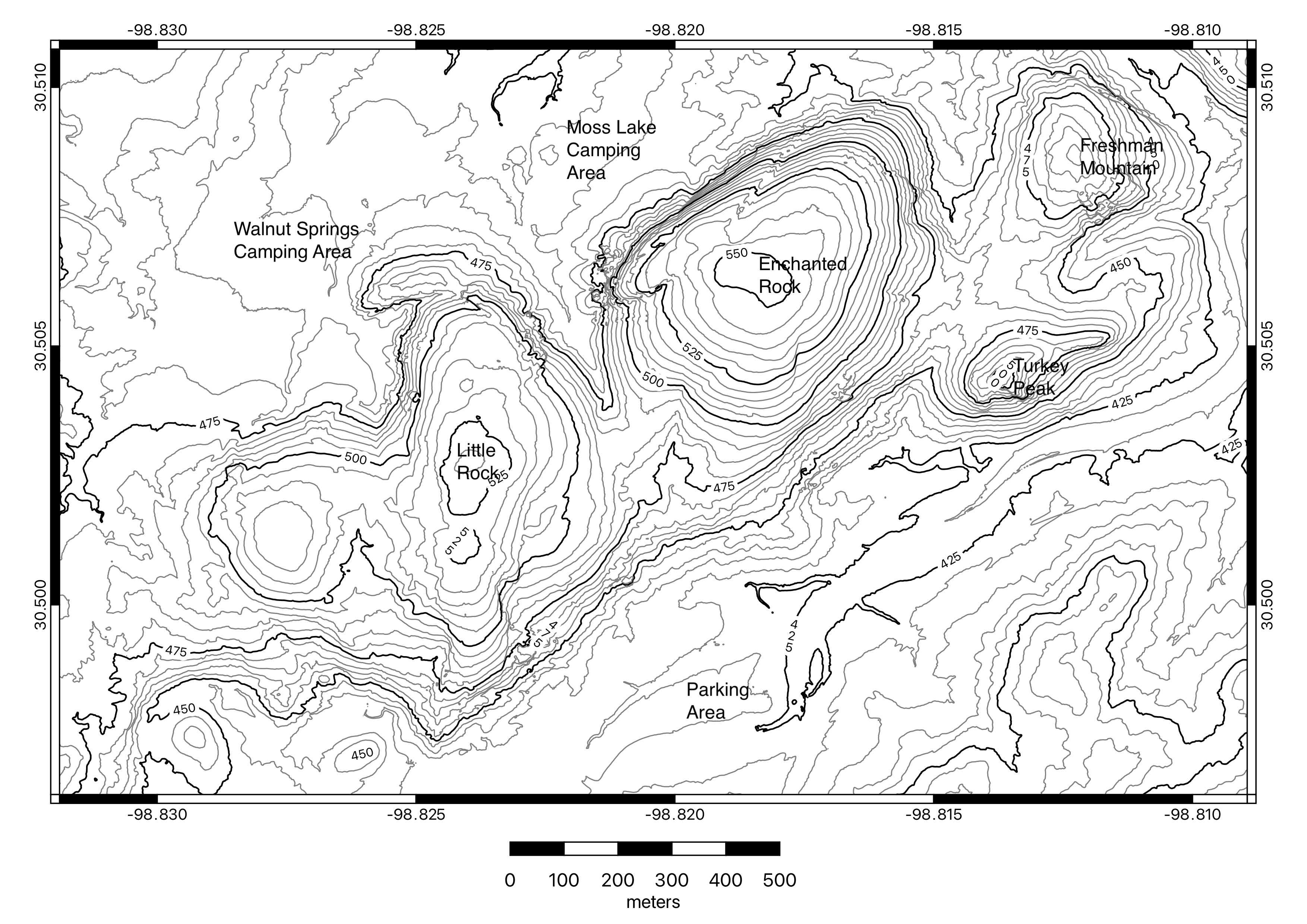
You and your friends are planning a hiking trip through Enchanted Rock State Natural Area (Figure 11.13). All the camping spots near the main parking lot are reserved. So, instead your group wants to camp in a backcountry at either Moss Lake or Walnut Springs. Some of your friends also want to go rock climbing.
-
- Estimate the elevation for the following points:
- Enchanted Rock: ____________________
- Little Rock: ____________________
- Parking Lot: ____________________
- There are two possible back country camp grounds at either Moss Lake or Walnut Springs. Chose one for your group. Draw two possible routes to this back country camping area from the parking lot. What is the length for each route?
- A: ____________________
- B: ____________________
- What is the elevation gain for each route:
- A: ____________________
- B: ____________________
- Which trip route would you take? A or B? Explain your reasoning.
- You and your friends decide to hike to the top of Enchanted Rock. Since the entire dome is just rock, you can go almost anywhere to get to the top. You want to take the path with the lowest slope because it will be easier. Draw the best path to take on Figure 11.13.
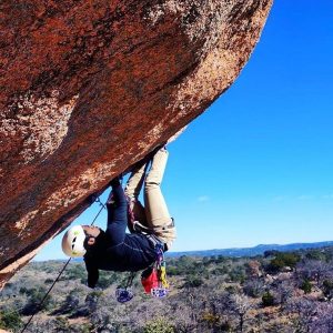
- You and your friends want to go rock climbing (Figure 11.14). They think there are several possible places with very steep topography. Which place has the steepest topography? Circle it on Figure 11.13.
- Estimate the elevation for the following points:
an instrument with a magnetized pointer that shows the direction of magnetic north and bearings from it.
map showing the arrangement of the natural and artificial physical features of an area
a line on a map joining points of equal height above or below sea level
a cone formed around a volcanic vent by fragments of lava ejected during an eruption. They typically only erupt once.
