
1.1 Overview of Microsoft Excel
Learning Objectives
- Examine the value of using Excel to make decisions.
- Learn how to start Excel.
- Become familiar with the Excel workbook.
- Understand how to navigate worksheets.
- Examine the Excel Ribbon.
- Examine the right-click menu options.
- Learn how to save workbooks.
- Examine the Status Bar.
- Become familiar with the features in the Excel Help window.
Microsoft® Office contains a variety of tools that help people accomplish many personal and professional objectives. Microsoft Excel is perhaps the most versatile and widely used of all the Office applications. No matter which career path you choose, you will likely need to use Excel to accomplish your professional objectives, some of which may occur daily. This chapter provides an overview of the Excel application along with an orientation for accessing the commands and features of an Excel workbook.
Making Decisions with Excel
Taking a very simple view, Excel is a tool that allows you to enter quantitative data into an electronic spreadsheet to apply one or many mathematical computations. These computations ultimately convert that quantitative data into information. The information produced in Excel can be used to make decisions in both professional and personal contexts. For example, employees can use Excel to determine how much inventory to buy for a clothing retailer, how much medication to administer to a patient, or how much money to spend to stay within a budget. With respect to personal decisions, you can use Excel to determine how much money you can spend on a house, how much you can spend on car lease payments, or how much you need to save to reach your retirement goals. We will demonstrate how you can use Excel to make these decisions and many more throughout this text.
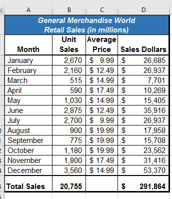
Figure 1.1 shows a completed Excel worksheet that will be constructed in this chapter. The information shown in this worksheet is top-line sales data for a hypothetical merchandise retail company. The worksheet data can help this retailer determine the number of salespeople needed for each month, how much inventory is needed to satisfy sales, and what types of products should be purchased.
Starting Excel
- Locate Excel on your computer.
- Click Microsoft Excel to launch the Excel application and present you with workbook options.
- Click the first option; “Blank Workbook”.
The Excel Workbook
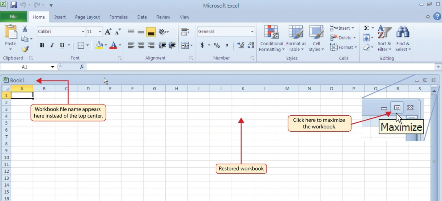
Once Excel is started, a blank workbook will open on your screen. A workbook is an Excel file that contains one or more worksheets (sometimes referred to as spreadsheets). Excel will assign a file name to the workbook, such as Book1, Book2, Book3, and so on, depending on how many new workbooks are opened. Figure 1.2 shows a blank workbook after starting Excel. Take some time to familiarize yourself with this screen. Your screen may be slightly different based on the version you’re using.
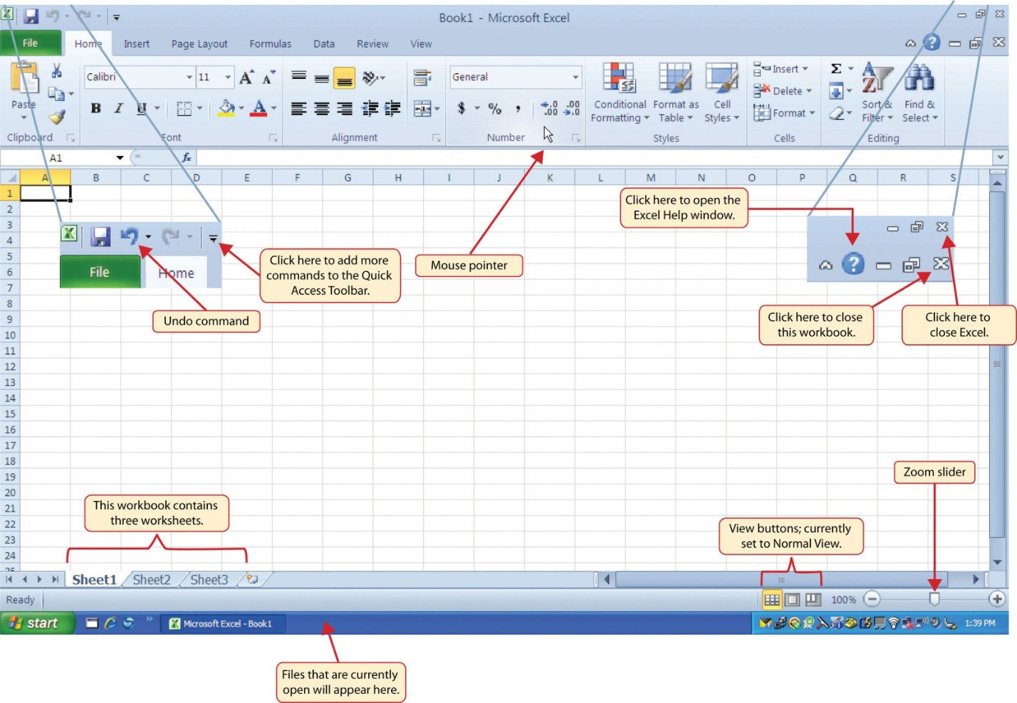
Your workbook should already be maximized (or shown at full size) once Excel is started, as shown in Figure 1.2. However, if your screen looks like Figure 1.3 after starting Excel, you should click the Maximize button, as shown in the figure.
Navigating Worksheets
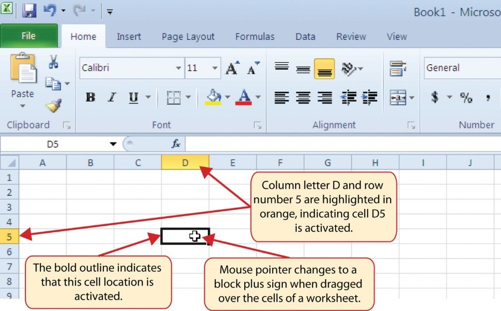
Data are entered and managed in an Excel worksheet. The worksheet contains several rectangles called cells for entering numeric and nonnumeric data. Each cell in an Excel worksheet contains an address, which is defined by a column letter followed by a row number. For example, the cell that is currently activated in Figure 1.3 is A1. This would be referred to as cell location A1 or cell reference A1. The following steps explain how you can navigate in an Excel worksheet:
- Place your mouse pointer over cell D5 and left click.
- Check to make sure column letter D and row number 5 are highlighted, as shown in Figure 1.4.
Note: Your highlighted column letter and row number may be different than the figure shown.
- Move the mouse pointer to cell A1.
- Click and hold the left mouse button and drag the mouse pointer back to cell D5.
- Release the left mouse button. You should see several cells highlighted, as shown in Figure 1.5.
This is referred to as a cell range and is documented as follows: A1:D5. Any two cell locations separated by a colon are known as a cell range. The first cell is the top left corner of the range and the second cell is the lower right corner of the range.
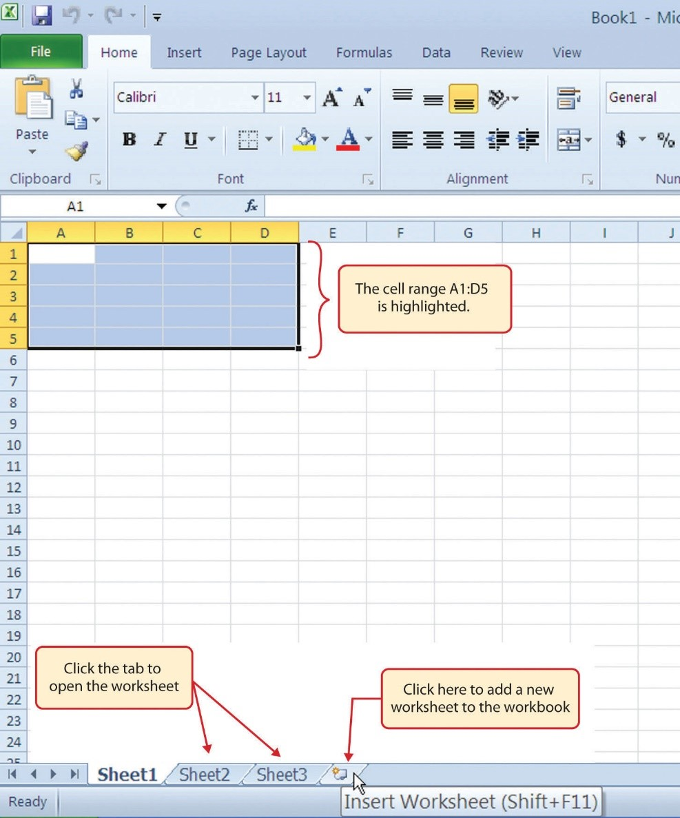
- At the bottom of the screen, you’ll see worksheets (Sheet 1, Sheet 2, Sheet 3 shown similar to how tabs look in a file folder). Depending on your version of Excel, you will see either three as displayed above or just one. If you only have one sheet, click the “Insert Worksheet” to add a worksheet.
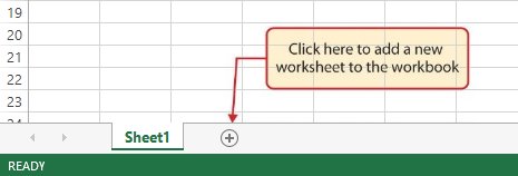
 Depending on your version, you instead may have a + sign; a click on the + adds an additional worksheet as well. This is how you open or add a worksheet within a workbook. You can also right-click the Sheet name and select Insert from the list of features that appear. Add another worksheet so that you have a total of three sheets displaying here.
 - Click the Sheet1 worksheet tab at the bottom of the worksheet to return to the worksheet shown in Figure 1.5.
Keyboard Shortcuts
Basic Worksheet Navigation
- Use the arrow keys on your keyboard to activate cells on the worksheet.
- Hold the SHIFT key and press the arrow keys on your keyboard to highlight a range of cells in a worksheet.
- Hold the CTRL key while pressing the PAGE DOWN or PAGE UP keys to open other worksheets in a workbook.
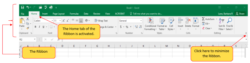
The Excel Ribbon
Excel’s features and commands are found in the Ribbon, which is the upper area of the Excel screen that contains several tabs running across the top. Each tab provides access to a different set of Excel commands. Figure 1.6 shows the commands available in the Home tab of the Ribbon. Table 1.1 “Command Overview for Each Tab of the Ribbon” provides an overview of the commands that are found in each tab of the Ribbon.
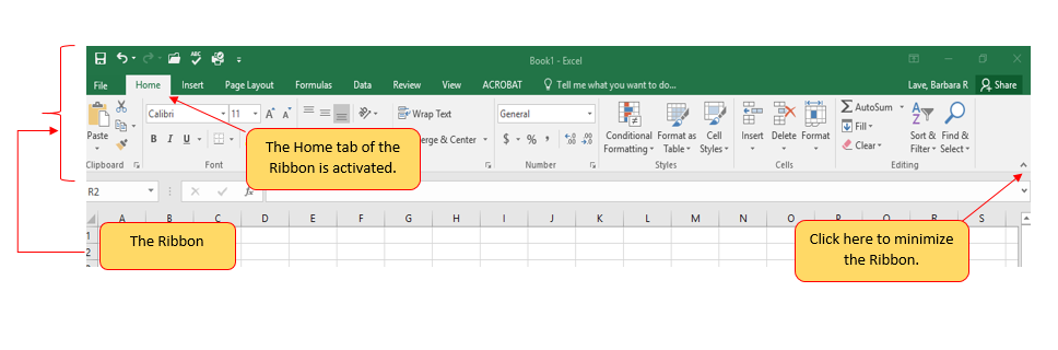
Table 1.1 Command Overview for Each Tab of the Ribbon
| Tab Name | Description of Commands |
| File | Also known as the Backstage view of the Excel workbook. Contains all commands for opening, closing, saving, and creating new Excel workbooks. Includes print commands, document properties, e-mailing options, and help features. The default settings and options are also found in this tab. |
| Home | Contains the most frequently used Excel commands. Formatting commands are found in this tab along with commands for cutting, copying, pasting, and for inserting and deleting rows and columns. |
| Insert | Used to insert objects such as charts, pictures, shapes, PivotTables, Internet links, symbols, or text boxes. |
| Page Layout | Contains commands used to prepare a worksheet for printing. Also includes commands used to show and print the gridlines on a worksheet. |
| Formulas | Includes commands for adding mathematical functions to a worksheet. Also contains tools for auditing mathematical formulas. |
| Data | Used when working with external data sources such as Microsoft® Access®, text files, or the Internet. Also contains sorting commands and access to scenario tools. |
| Review | Includes Spelling and Track Changes features. Also contains protection features to password protect worksheets or workbooks. |
| View | Used to adjust the visual appearance of a workbook. Common commands include the Zoom and Page Layout view. |
The Ribbon shown in Figure 1.6 is full, or maximized. The benefit of having a full Ribbon is that the commands are always visible while you are developing a worksheet. However, depending on the screen dimensions of your computer, you may find that the Ribbon takes up too much vertical space on your worksheet. If this is the case, you can minimize the Ribbon by clicking the button shown in Figure 1.6. When minimized, the Ribbon will show only the tabs and not the command buttons. When you click on a tab, the command buttons will appear until you select a command or click anywhere on your worksheet.
Keyboard Shortcuts
Minimizing or Maximizing the Ribbon
- Hold down the CTRL key and press the F1 key.
- Hold down the CTRL key and press the F1 key again to maximize the Ribbon.
Quick Access Toolbar and Right-Click Menu
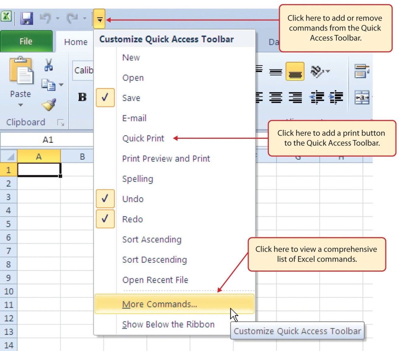
The Quick Access Toolbar is found at the upper left side of the Excel screen above the Ribbon, as shown in Figure 1.7. This area provides access to the most frequently used commands, such as Save and Undo. You can customize the Quick Access Toolbar by adding commands that you use on a regular basis. By placing these commands in the Quick Access Toolbar, you do not have to navigate through the Ribbon to find them. To customize the Quick Access Toolbar, click the down arrow as shown in Figure 1.7. This will open a menu of commands that you can add to the Quick Access Toolbar. If you do not see the command you are looking for on the list, select the More Commands option.
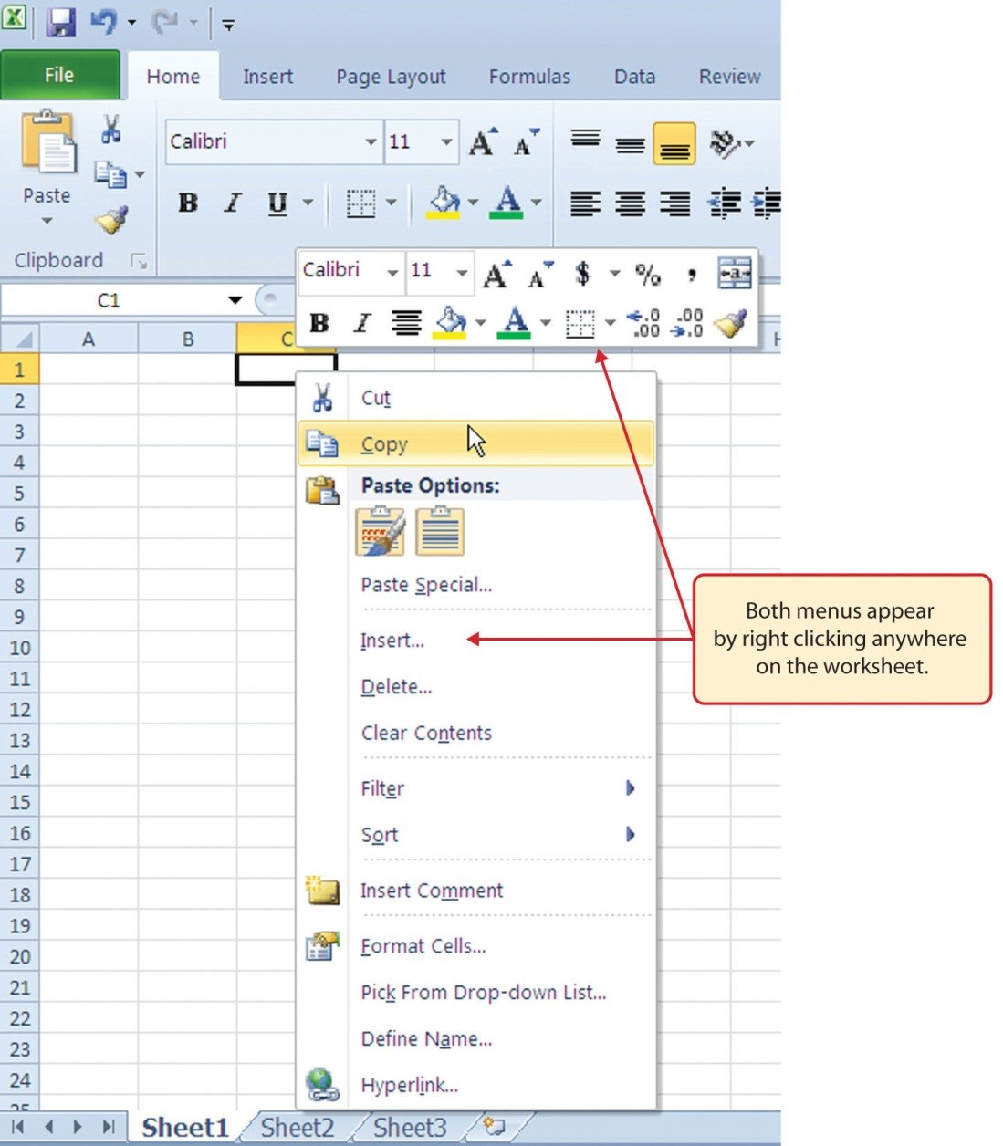
In addition to the Ribbon and Quick Access Toolbar, you can also access commands by right clicking anywhere on the worksheet. Figure 1.8 shows an example of the commands available in the right-click menu.
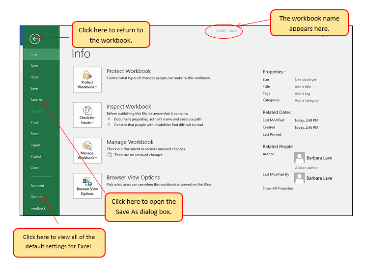
The File Tab
The File tab is also known as the Backstage view of the workbook. It contains a variety of features and commands related to the workbook that is currently open, new workbooks, or workbooks stored in other locations on your computer or network. Figure 1.9 shows the options available in the File tab or Backstage view. To leave the Backstage view and return to the worksheet, click the arrow in the upper left-hand corner as shown below.
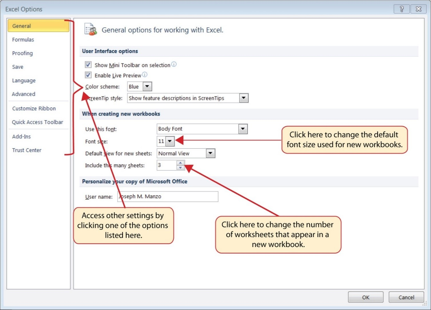
Included in the File tab are the default settings for the Excel application that can be accessed and modified by clicking the Options button. Figure 1.10 shows the Excel Options window, which gives you access to settings such as the default font style, font size, and the number of worksheets that appear in new workbooks.
Saving Workbooks (Save As)
Once you create a new workbook, you will need to change the file name and choose a location on your computer or network to save that file. It is important to remember where you save this workbook on your computer or network as you will be using this file in the Section 1.2 “Entering, Editing, and Managing Data” to construct the workbook shown in Figure 1.1. The process of saving can be different with different versions of Excel. Please be sure you follow the steps for the version of Excel you are using. The following steps explain how to save a new workbook and assign it a file name.
Saving Workbooks in Excel 2013
- If you have not done so already, open a blank workbook in Excel.
- When saving your workbook for the first time, click the File tab.
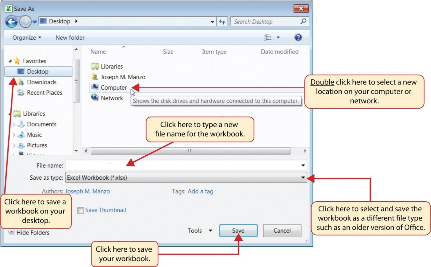
- Click the Save As button in the upper left side of the Backstage view window. This will open the Save As dialog box, as shown in Figure 1.11.
- Click in the File Name box at the bottom of the Save As dialog box and use the BACKSPACE key to remove the current default name of the workbook.
- Type the file name: CH1 GMW Sales Data.
- Click the Desktop button on the left side of the Save As dialog box if you wish to save this file on your desktop. If you want to save this workbook in a different location, such as a USB drive, select your preferred location.
- Click the Save button on the lower right side of the Save As dialog box.
- As you continue to work on your workbook, you will want to Save frequently by clicking either the Save button on the Home ribbon; or by selecting the Save option from the File menu.
Saving Workbooks in Excel 2016
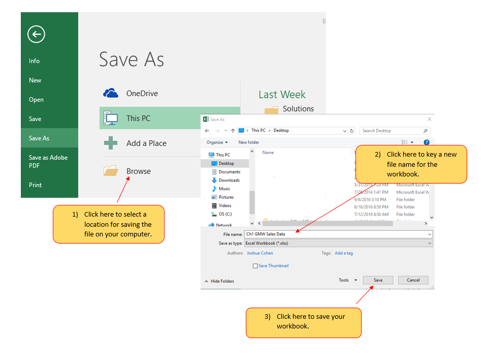
- If you have not done so already, open a blank workbook in Excel.
- Click the File tab and then the Save As button in the left side of the Backstage view window. This will open the Save As dialog box.
- Determine a location for saving on your computer by clicking Browse on the left side to open the Save As dialog box.
- Click in the File Name box near the bottom of the Save As dialog box. Type the new file name: CH1 GMW Sales Data
- Review the settings in the screen for correctness and click the Save button.
Keyboard Shortcuts
“Save” and “Save As”
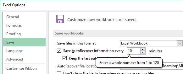
- CTRL+S will call up the Save As dialog box. If you have already saved your file, CTRL+S will save your progress from the last auto-save point. All Office applications will Save AutoRecover information at specific intervals (usually every 10 minutes), you can edit this setting to 5 minutes or to every minute under File > Options > Excel Options > Save workbooks.
- Press the F12 key and use the tab and arrow keys to navigate around the Save As dialog box. Use the ENTER key to make a selection.
- Or press the ALT key on your keyboard. You will see letters and numbers, called Key Tips, appear on the Ribbon. Press the F key on your keyboard for the File tab and then the A key. This will open the Save As dialog box.
Skill Refresher
Saving Workbooks (Save As)
- Click the File tab on the Ribbon.
- Click the Save As option.
- Select a location on your PC.
- Click in the File name box and type a new file name if needed.
- Click the down arrow next to the “Save as type” box and select the appropriate file type if needed.
- Click the Save button.
The Status Bar
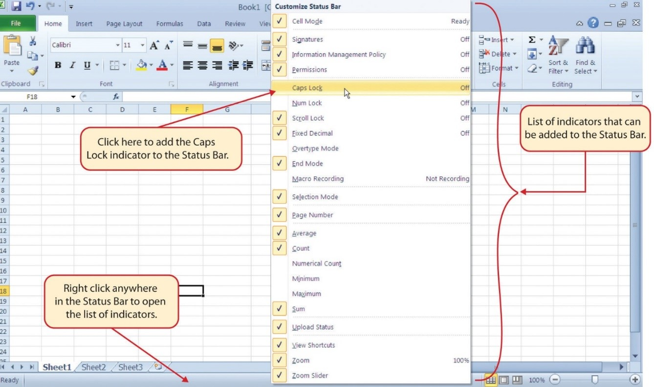
The Status Bar is located below the worksheet tabs on the Excel screen (see Figure 1.13). It displays a variety of information, such as the status of certain keys on your keyboard (e.g., CAPS LOCK), the available views for a workbook, the magnification of the screen, and mathematical functions that can be performed when data are highlighted on a worksheet. You can customize the Status Bar as follows:
- Place the mouse pointer over any area of the Status Bar and right click to display the “Customize Status Bar” list of options (see Figure 1.13).
- Select the Caps Lock option from the menu (see Figure 1.13).
- Press the CAPS LOCK key on your keyboard. You will see the Caps Lock indicator on the lower right side of the Status Bar.
- Press the CAPS LOCK on your keyboard again. The indicator on the Status Bar goes away.
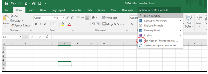
Excel Help
The Help feature provides extensive information about the Excel application. Although some of this information may be stored on your computer, the Help window will automatically connect to the Internet, if you have a live connection, to provide you with resources that can answer most of your questions. You can open the Excel Help window by clicking the question mark in the upper right area of the screen or ribbon. With newer versions of Excel, use the query box to enter your question and select from helpful option links or select the question mark from the dropdown list to launch Excel Help windows.
Keyboard Shortcuts
Excel Help
- Press the F1 key on your keyboard.
Key Takeaways
- Excel is a powerful tool for processing data for the purposes of making decisions.
- You can find Excel commands throughout the tabs in the Ribbon.
- You can customize the Quick Access Toolbar by adding commands you frequently use.
- You can add or remove the information that is displayed on the Status Bar.
- The Help window provides you with extensive information about Excel.
Attribution
Adapted by Barbara Lave from How to Use Microsoft Excel: The Careers in Practice Series, adapted by The Saylor Foundation without attribution as requested by the work’s original creator or licensee, and licensed under CC BY-NC-SA 3.0.
