2.2 Creating & Auditing Complex Formulas
Creating Complex Formulas (Controlling the Order of Operations)
The next formula to be added to the Personal Budget workbook is the percent change over last year. This formula determines the difference between the values in the LY (Last Year) Spend column and shows the difference in terms of a percentage. This requires that the order of mathematical operations be controlled to get an accurate result. Table 2.3 shows the standard order of operations for a typical formula. To change the order of operations shown in the table, we use parentheses to process certain mathematical calculations first. This formula is added to the worksheet as follows:
- Click cell F3 in the Budget Detail worksheet.
- Type an equal sign =.
- Type an open parenthesis (.
- Click cell D3. This will add a cell reference to cell D3 to the formula. When building formulas, you can click cell locations instead of typing them.
- Type a minus sign −.
- Click cell E3 to add this cell reference to the formula.
- Type a closing parenthesis ).
- Type the slash / symbol for division.
- Click cell E3. This completes the formula that will calculate the percent change of last year’s actual spent dollars vs. this year’s budgeted spend dollars (see Figure 2.6).
- Press the ENTER key.
- Click cell F3 to activate it.
- Place the mouse pointer over the Auto Fill Handle.
- When the mouse pointer turns from a white block plus sign to a black plus sign, click and drag down to cell F11. This pastes the formula into the range F4:F11.
Table 2.3 Standard Order of Mathematical Operations
| Symbol | Order |
| ( ) | Override Standard Order: Any mathematical computations placed in parentheses are performed first and override the standard order of operations. If there are layers of parentheses used in a formula, Excel computes the innermost parentheses first and the outermost parentheses last. |
| ^ | First: Excel executes any exponential computations first. |
| * or / | Second: Excel performs any multiplication or division computations second. When there are multiple instances of these computations in a formula, they are executed in order from left to right. |
| + or − | Third: Excel performs any addition or subtraction computations third. When there are multiple instances of these computations in a formula, they are executed in order from left to right. |
Figure 2.6 shows the formula that was added to the Budget Detail worksheet to calculate the percent change in spending. The parentheses were added to this formula to control the order of operations. Any mathematical computations placed in parentheses are executed first before the standard order of mathematical operations (see Table 2.3). In this case, if parentheses were not used, Excel would produce an erroneous result for this worksheet.
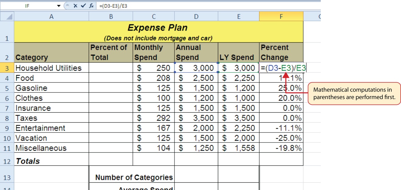
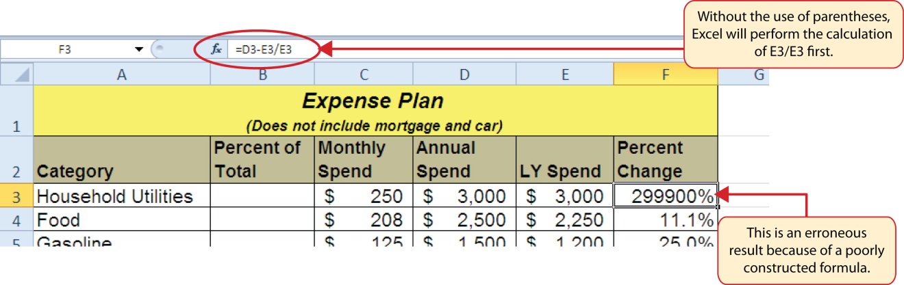
Figure 2.7 shows the result of the percent change formula if the parentheses are removed. The formula produces a result of a 299900% increase. Since there is no change between the LY spend and the budget Annual Spend, the result should be 0%. However, without the parentheses, Excel is following the standard order of operations. This means the value in cell E3 will be divided by E3 first (3,000/3,000), which is 1. Then, the value of 1 will be subtracted from the value in cell D3 (3,000−1), which is 2,999. Since cell F3 is formatted as a percentage, Excel expresses the output as an increase of 299900%.
Integrity Check
Does the Output of Your Formula Make Sense?
It is important to note that the accuracy of the output produced by a formula depends on how it is constructed. Therefore, always check the result of your formula to see whether it makes sense with data in your worksheet. As shown in Figure 2.7, a poorly constructed formula can give you an inaccurate result. In other words, you can see that there is no change between the Annual Spend and LY Spend for Household Utilities. Therefore, the result of the formula should be 0%. However, since the parentheses were removed in this case, the formula is clearly producing an erroneous result.
Skill Refresher
Formulas
- Type an equal sign =.
- Click or type a cell location. If using constants, type a number.
- Type a mathematical operator.
- Click or type a cell location. If using constants, type a number.
- Use parentheses where necessary to control the order of operations.
- Press the ENTER key.
Auditing Formulas
Excel provides a few tools that you can use to review the formulas entered into a worksheet. For example, instead of showing the outputs for the formulas used in a worksheet, you can have Excel show the formula as it was entered in the cell locations. This is demonstrated as follows:
- With the Budget Detail worksheet open, click the Formulas tab of the Ribbon.
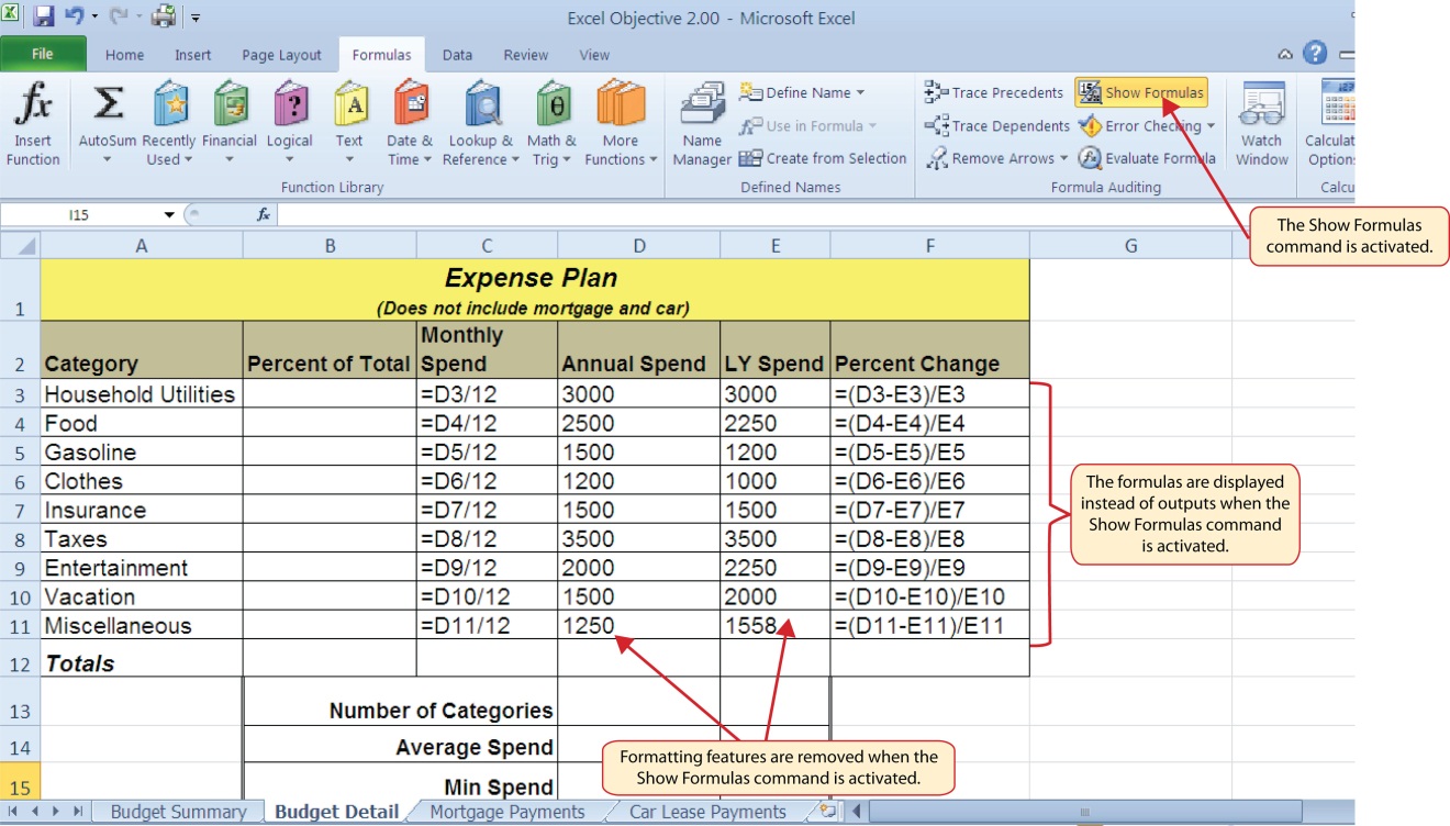
- Click the Show Formulas button in the Formula Auditing group of commands. This displays the formulas in the worksheet instead of showing the mathematical outputs.
- Click the Show Formulas button again. The worksheet returns to showing the output of the formulas.
Figure 2.8 shows the Budget Detail worksheet after activating the Show Formulas command in the Formulas tab of the Ribbon. As shown in the figure, this command allows you to view and check all the formulas in a worksheet without having to click each cell individually. After activating this command, the column widths in your worksheet increase significantly. The column widths were adjusted for the worksheet shown in Figure 2.8 so all columns can be seen. The column widths return to their previous width when the Show Formulas command is deactivated.
Skill Refresher
Show Formulas
- Click the Formulas tab on the Ribbon.
- Click the Show Formulas button in the Formula Auditing group of commands.
- Click the Show Formulas button again to show formula outputs.
Keyboard Shortcuts
Show Formulas
- Hold down the CTRL key while pressing the accent symbol `.
Two other tools in the Formula Auditing group of commands are the Trace Precedents and Trace Dependents commands. These commands are used to trace the cell references used in a formula. A precedent cell is a cell whose value is used in other cells. The Trace Precedents command shows an arrow to indicate the cells or ranges (precedents) which affect the active cell’s value. A dependent cell is a cell whose value depends on the values of other cells in the workbook. The Trace Dependents command shows where any given cell is referenced in a formula. The following is a demonstration of these commands:
- Click cell D3 in the Budget Detail worksheet.
- Click the Trace Dependents button in the Formula Auditing group of commands in the Formulas tab of the Ribbon. A double blue arrow appears, pointing to cell locations C3 and F3 (see Figure 2.9). This indicates that cell D3 is referenced in formulas that are entered in cells C3 and F3.
- Click the Remove Arrows command in the Formula Auditing group of commands in the Formulas tab of the Ribbon. This removes the Trace Dependents arrow.
- Click cell F3 in the Budget Detail worksheet.
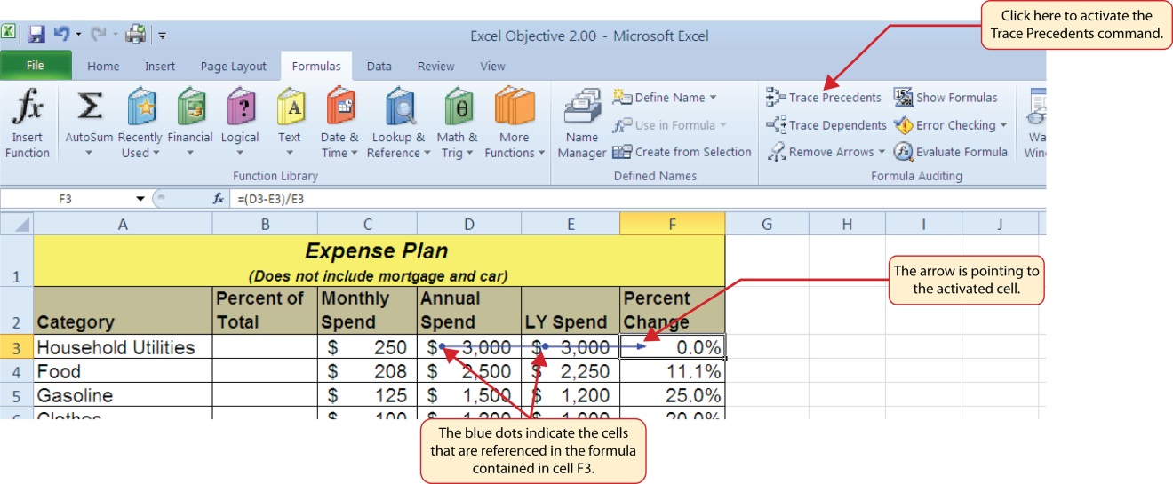
- Click the Trace Precedents button in the Formula Auditing group of commands in the Formulas tab of the Ribbon. A blue arrow running through cells D3 and E3 and pointing to cell F3 appears (see Figure 2.10). This indicates that cells D3 and E3 are references in a formula entered in cell F3.
- Click the Remove Arrows command in the Formula Auditing group of commands in the Formulas tab of the Ribbon. This removes the Trace Precedents arrow.
- Save the Ch2 Personal Budget file.
Figure 2.9 shows the Trace Dependents arrow on the Budget Detail worksheet. The blue dot represents the activated cell. The arrows indicate where the cell is referenced in formulas.
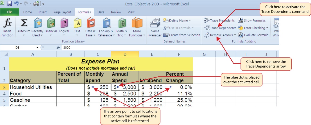
Figure 2.10 shows the Trace Precedents arrow on the Budget Detail worksheet. The blue dots on this arrow indicate the cells that are referenced in the formula contained in the activated cell. The arrow is pointing to the activated cell location that contains the formula.