
3.3 The VLOOKUP Function
Lookup & Reference Functions automate the process of returning values that match your criteria. This means, that if you have a table that is missing some values, but you have another table that has these, you can use it to cross-reference and match what is missing from your original table. Excel will find and return values for you quickly and effectively without you having to manually enter data.
In a lot of ways, this is very similar to looking up information in an online phone book or directory. A directory is a common way of storing corresponding pieces of data in alphabetical or numerical order. There are names or ID numbers or product codes that are used to signify an entity you put in a prominent place, usually in the first column of a table. This column is followed by attributes or characteristics related to that entity, person or product. In your grade book, you are an entity signified by your name, your assignment scores are attributes that describe your performance. In your bank records, your credit card number or social security number describes you as an entity, your purchase date, the purchase amount, the place where you purchased an item are attributes that describe your spending habits.
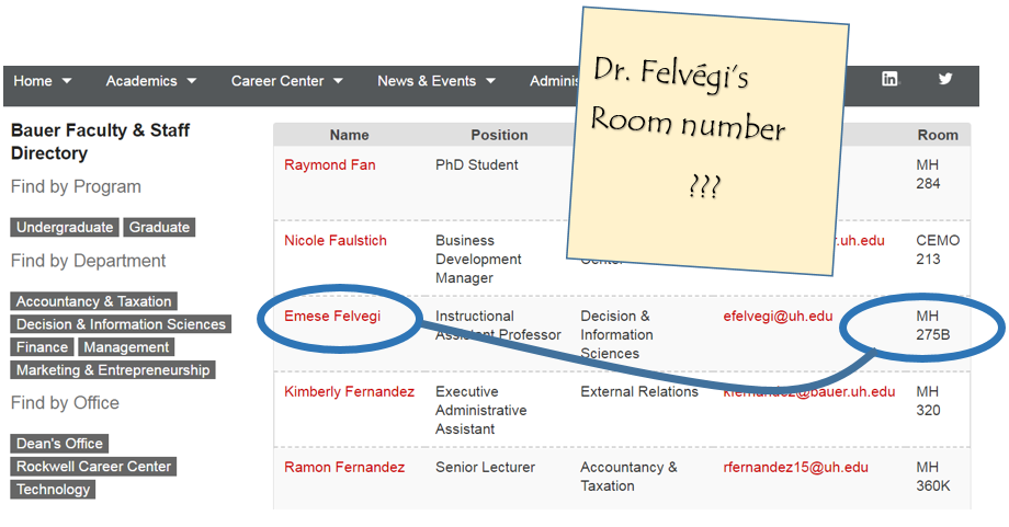
Let’s look at the table below to see how we generally find things in lists if we look for one piece of data. If you know your professor’s (entity) name (attribute) and you want to look up their Room number (another attribute). You go to the directory that lists all of your faculty and staff, find your professor’s name on that list, then go to the column that has their Room number and then write it on a Post It note or in your class notebook.
We can easily Google a single piece of data. However, VLOOKUP will let us automate this process with a few hundred or a few hundreds of thousands of pieces of data that are stored in a column or vertical structure. The overview of the syntax and how the process altogether works in Excel is as follows.
=VLOOKUP(lookup_value, table_array, col_index_num, [range_lookup])
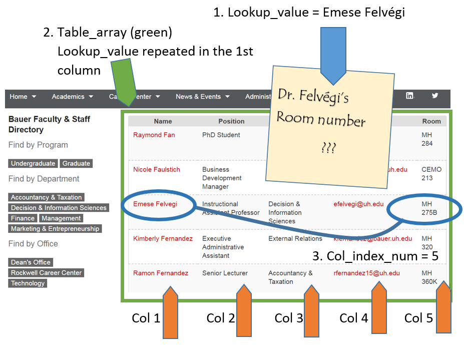
- Lookup_value – It is the piece of data we know, the Professor’s name on our original Post It note.
- Table_array – This is the range that contains the value that has the data we are looking for and starts with your Lookup_value. In our case with the directory, it’s the table that starts with the Professor’s name and ends with the column where the room number is in.
- Col_index_number – This is the column in the table array range that includes the information that we are looking up. In our case, the Room is in the 5th column of the table array range.
- Range_lookup – There are two options with this argument in our formula: approximate match or exact match. The default value of TRUE means that Excel will look for an approximate match for your value in a range of values and return the lower corresponding value. If you do not enter anything for this argument, it will return based on the default. However, if you are looking for something definite, the FALSE option will return an exact match. Your professors are not interchangeable, so you will need an exact match.
Let’s try this process next on our grade book from the CH3 practice.
USING VLOOKUP to return grades
For our chapter grade book example, we need to know what grade each student is getting based on their percentage score. You will find the table that defines the scores and the grades in A28:B32.
There are four pieces of information that you will need in order to build the VLOOKUP syntax. These are the four arguments of a VLOOKUP function:
- The value you want to look up, also called the Lookup_value. In our example, the lookup value will be the student’s percentage score in column P.
- The Table_array is the range (table) where the lookup values and the values you want returned by the function are located. In our example, this is the table of percentages and corresponding letter grades in the range A28:B32. The lookup value should always be in the first column in the table array for VLOOKUP to work correctly. For example, in our table_array the lookup value is in cell A28, so the range should start with A.
- The Col_index_num is the column number in the range that contains the value to return. In our example, when you specify A28:B32 as the Table_array range, you should count A as the first column (1), B as the second column (2), and so on. You will enter the appropriate column number in this box as 1, 2, or 3 and so on.
- In the Range_lookup, you can optionally specify TRUE if you want an approximate match or FALSE if you want an exact match of the return value. If you leave this blank, the default value will always be TRUE, or approximate match.
Let’s create the VLOOKUP to display the correct Letter Grade in column R.
- Make sure that R5 is your active cell.
- On the Formulas tab, in the Function Library, find the VLOOKUP function on the Lookup & Reference pull-down menu (see Figure 3.12).
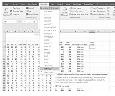
Figure 3.12 VLOOKUP Function - Fill in the dialog box so that it looks like the image in Figure 3.13.
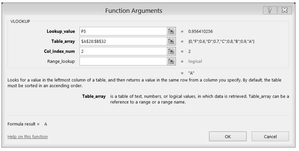
- Lookup_value – In this case, we will use the Percentage score. So, P5 for the first look up value.
- Table_array – This is the range that contains the value you want returned by the function. In this case, that range is A28:B32. Note that this range does NOT include the label in row 27; just the actual data. The cell references for the Table_array need to be absolute – $A$28:$B$32. When we copy this function to the other cells, we do not want these cell references to change. It should always be $A$28:$B$32.
- Col_index_number – This is the column in the table array range that includes the information that we are looking up. In our case, the actual grades are in the 2nd column of the range. So, the column index will be 2.
- Range_lookup – In some cases, you will need something in the Range_lookup box. Since we are looking for an approximate match for the percentages, we want the default value of TRUE, so we do not need to enter anything for this argument.
- While you are in the dialog box, be sure to look at all the helpful definitions that Excel offers.
- When you have filled in the dialog box, press OK.
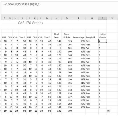
- The calculation you will see in the formula bar is: =VLOOKUP(P5,$A$28:$B$32,2)
- Use the fill handle to copy the function down through row 24. The results displayed should match Figure 3.14.
Note: What if it didn’t work? What if you get a result different from the one predicted? In this case, either you have made a previous error, resulting in different % scores than this exercise anticipated, or you made a mistake entering your VLOOKUP function.
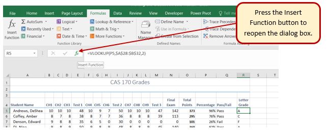
To make repairs in the function, make sure that R5 is your active cell. On the Formula bar, press the Insert Function button (see Figure 3.15). That will reopen the dialog box so you can make your repairs. Did you forget to make the cell references for the Table_array absolute? Did you use the wrong cell for the Lookup_value? Press OK when you are done and recopy the corrected function.
“3.3 VLOOKUP” by Emese Felvégi, Diane Shingledecker, PCC.EDU is licensed under CC BY 4.0.
