
1.2 Entering, Editing, and Managing Data
Learning Objectives
- Understand how to enter data into a worksheet.
- Examine how to edit data in a worksheet.
- Examine how Auto Fill is used when entering data.
- Understand how to delete data from a worksheet and use the Undo command.
- Examine how to adjust column widths and row heights in a worksheet.
- Understand how to hide columns and rows in a worksheet.
- Examine how to insert columns and rows into a worksheet.
- Understand how to delete columns and rows from a worksheet.
- Learn how to move data to different locations in a worksheet.
In this section, we will begin the development of the workbook shown in Figure 1.1. The skills covered in this section are typically used in the early stages of developing one or more worksheets in a workbook.
Entering Data
You will begin building the workbook shown in Figure 1.1 by manually entering data into the worksheet. The following steps explain how the column headings in Row 2 are typed into the worksheet:
- Click cell location A2 on the worksheet.
- Type the word Month.
- Press the RIGHT ARROW key. This will enter the word into cell A2 and activate the next cell to the right.
- Type Unit Sales and press the RIGHT ARROW key.
- Repeat step 4 for the words Average Price and then again for Sales Dollars.
Figure 1.15 shows how your worksheet should appear after you have typed the column headings into Row 2. Notice that the word Price in cell location C2 is not visible. This is because the column is too narrow to fit the entry you typed. We will examine formatting techniques to correct this problem in the next section.
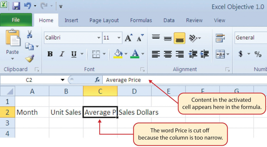
Integrity Check
Column Headings
It is critical to include column headings that accurately describe the data in each column of a worksheet. In professional environments, you will likely be sharing Excel workbooks with coworkers. Good column headings reduce the chance of someone misinterpreting the data contained in a worksheet, which could lead to costly errors depending on your career.
- Click cell location B3.
- Type the number 2670 and press the ENTER key. After you press the ENTER key, cell B4 will be activated. Using the ENTER key is an efficient way to enter data vertically down a column.
- Enter the following numbers in cells B4 through B14: 2160, 515, 590, 1030, 2875, 2700, 900, 775, 1180, 1800, and 3560.
- Click cell location C3.
- Type the number 9.99 and press the ENTER key.
- Enter the following numbers in cells C4 through C14: 12.49, 14.99, 17.49, 14.99, 12.49, 9.99, 19.99, 19.99, 19.99, 17.49, and 14.99.
- Activate cell location D3.
- Type the number 26685 and press the ENTER key.
- Enter the following numbers in cells D4 through D14: 26937, 7701, 10269, 15405, 35916, 26937, 17958, 15708, 23562, 31416, and 53370.
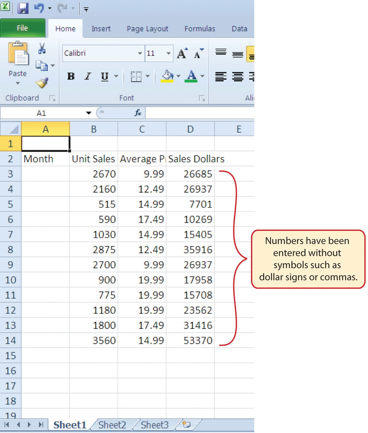
- When finished, check that the data you entered matches Figure 1.16.
Why?
Avoid Formatting Symbols When Entering Numbers
When typing numbers into an Excel worksheet, it is best to avoid adding any formatting symbols such as dollar signs and commas. Although Excel allows you to add these symbols while typing numbers, it slows down the process of entering data. It is more efficient to use Excel’s formatting features to add these symbols to numbers after you type them into a worksheet.
Integrity Check
Data Entry
It is very important to proofread your worksheet carefully, especially when you have entered numbers. Transposing numbers when entering data manually into a worksheet is a common error. For example, the number 563 could be transposed to 536. Such errors can seriously compromise the integrity of your workbook.
Integrity Check
Figure 1.16 shows how your worksheet should appear after entering the data. Check your numbers carefully to make sure they are accurately entered into the worksheet.
Editing Data
Data that has been entered in a cell can be changed by double clicking the cell location or using the Formula Bar. You may have noticed that as you were typing data into a cell location, the data you typed appeared in the Formula Bar. The Formula Bar can be used for entering data into cells as well as for editing data that already exists in a cell. The following steps provide an example of entering and then editing data that has been entered into a cell location:
- Click cell A15 in the Sheet1 worksheet.
- Type the abbreviation Tot and press the ENTER key.
- Click cell A15.
- Move the mouse pointer up to the Formula Bar. You will see the pointer turn into a cursor. Move the cursor to the end of the abbreviation Tot and left click.
- Type the letters al to complete the word Total.
- Click the checkmark to the left of the Formula Bar (see Figure 1.17). This will enter the change into the cell.
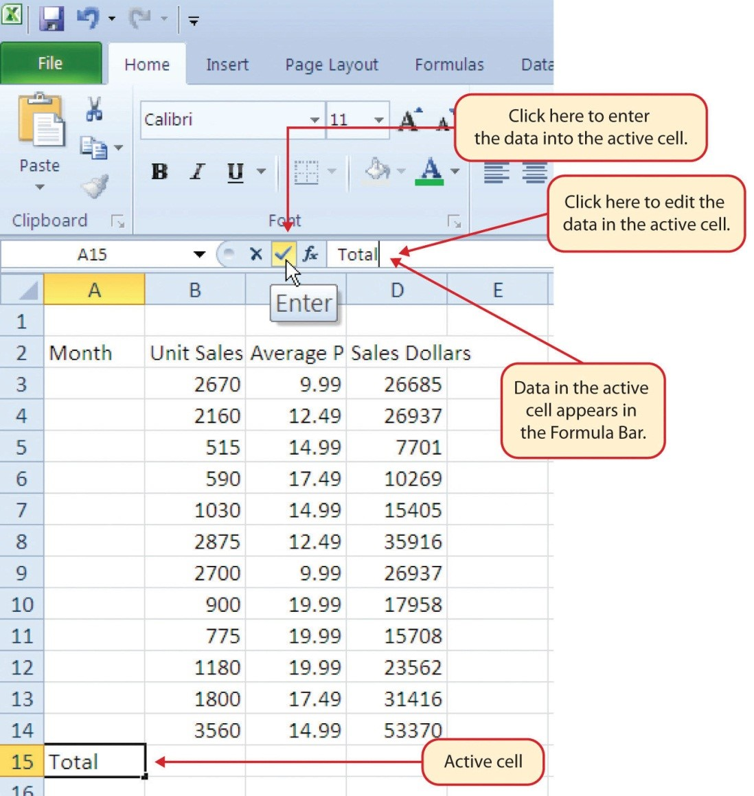
Figure 1.17 Using the Formula Bar to Edit and Enter Data - Double click cell A15.
- Add a space after the word Total and type the word Sales.
- Press the ENTER key.
Keyboard Shortcuts
Editing Data in a Cell
- Activate the cell that is to be edited and press the F2 key on your keyboard.
Auto Fill
The Auto Fill feature is a valuable tool when manually entering data into a worksheet. This feature has many uses, but it is most beneficial when you are entering data in a defined sequence, such as the numbers 2, 4, 6, 8, and so on, or nonnumeric data such as the days of the week or months of the year. The following steps demonstrate how Auto Fill can be used to enter the months of the year in Column A:
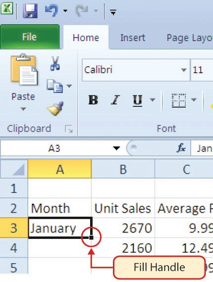
- Click cell A3 in the Sheet1 worksheet.
- Type the word January and press the ENTER key.
- Activate cell A3 again.
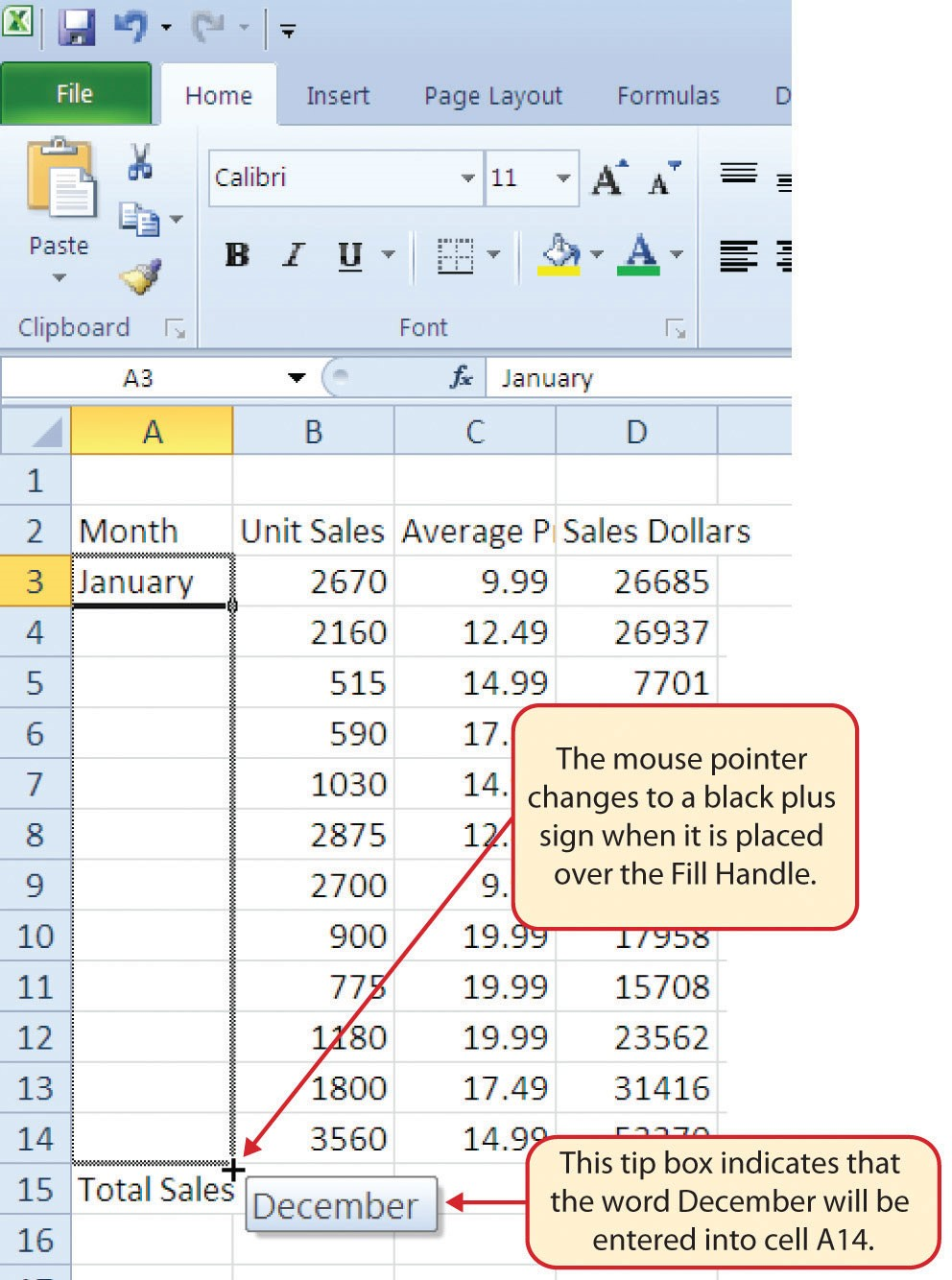
- Move the mouse pointer to the lower right corner of cell A3. You will see a small square in this corner of the cell; this is called the Fill Handle (See Figure 1.18) When the mouse pointer gets close to the Fill Handle, the white block plus sign will turn into a black plus sign.
Left click and drag the Fill Handle to cell A14. Notice that the Auto Fill tip box indicates what month will be placed into each cell (see Figure 1.19). Release the left mouse button when the tip box reads “December.”
Once you release the left mouse button, all twelve months of the year should appear in the cell range A3:A14, as shown in Figure 1.20. You will also see the Auto Fill Options button. By clicking this button, you have several options for inserting data into a group of cells.
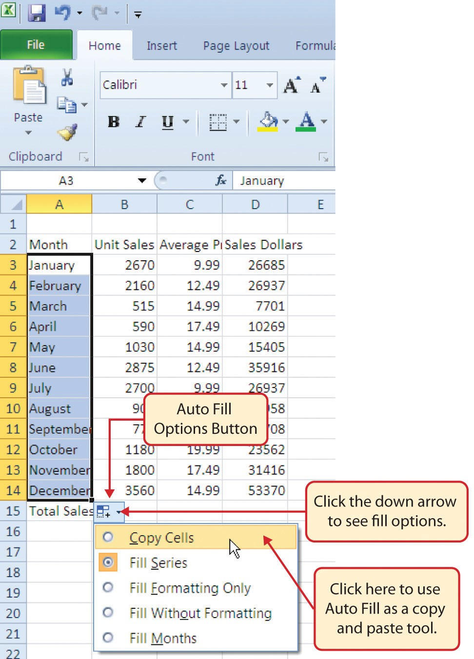
- Click the Auto Fill Options button.
- Click the Copy Cells option. This will change the months in the range A4:A14 to January.
- Click the Auto Fill Options button again.
- Click the Fill Months option to return the months of the year to the cell range A4:A14. The Fill Series option will provide the same result.
Deleting Data and the Undo Command
There are several methods for removing data from a worksheet, a few of which are demonstrated here. With each method, you use the Undo command. This is a helpful command in the event you mistakenly remove data from your worksheet. The following steps demonstrate how you can delete data from a cell or range of cells:
- Click cell C2 by placing the mouse pointer over the cell and clicking the left mouse button.
- Press the DELETE key on your keyboard. This removes the contents of the cell.
- Highlight the range C3:C14 by placing the mouse pointer over cell C3. Then left click and drag the mouse pointer down to cell C14.
- Place the mouse pointer over the Fill Handle. You will see the white block plus sign change to a black plus sign.
- Click and drag the mouse pointer up to cell C3 (see Figure 1.21). Release the mouse button. The contents in the range C3:C14 will be removed.
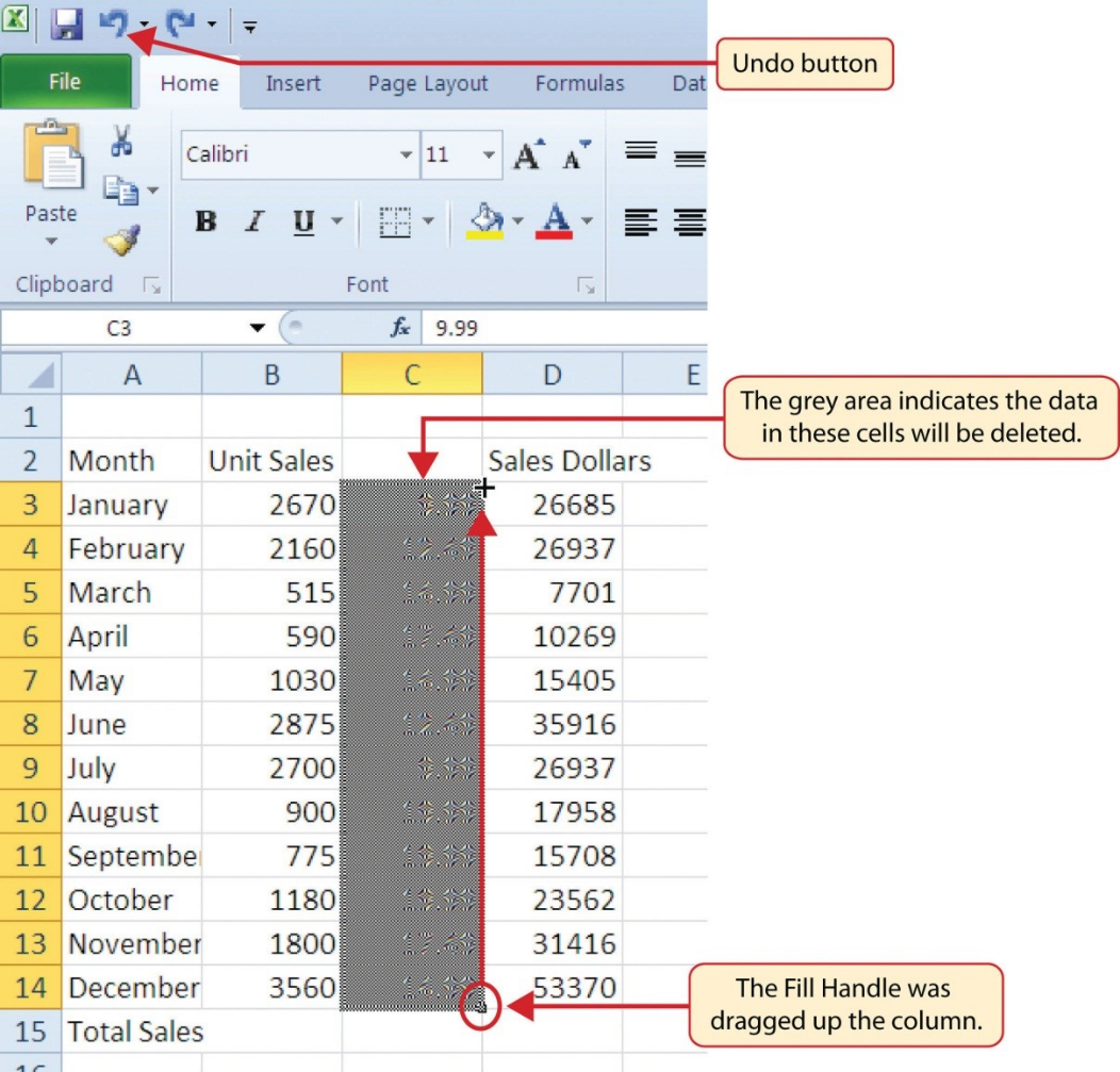
- Click the Undo button in the Quick Access Toolbar (see Figure 1.2). This should replace the data in the range C3:C14.
- Click the Undo button again. This should replace the data in cell C2.
Keyboard Shortcuts
Undo Command
- Hold down the CTRL key while pressing the letter Z on your keyboard.
- Highlight the range C2:C14 by placing the mouse pointer over cell C2. Then left click and drag the mouse pointer down to cell C14.
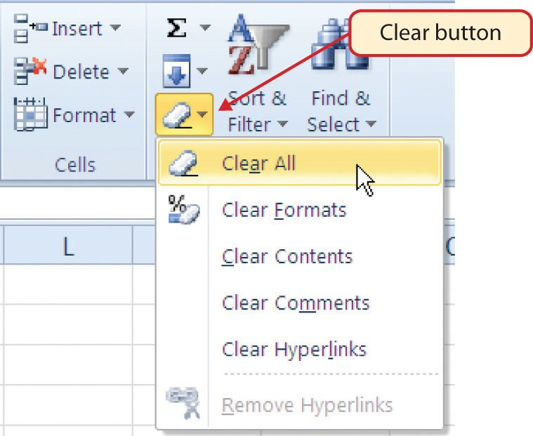
- Click the Clear button in the Home tab of the Ribbon, which is next to the Cells group of commands (see Figure 1.22). This opens a drop-down menu that contains several options for removing or clearing data from a cell. Notice that you also have options for clearing just the formats in a cell or the hyperlinks in a cell.
- Click the Clear All option. This removes the data in the cell range.
- Click the Undo button. This replaces the data in the range C2:C14.
Adjusting Columns and Rows
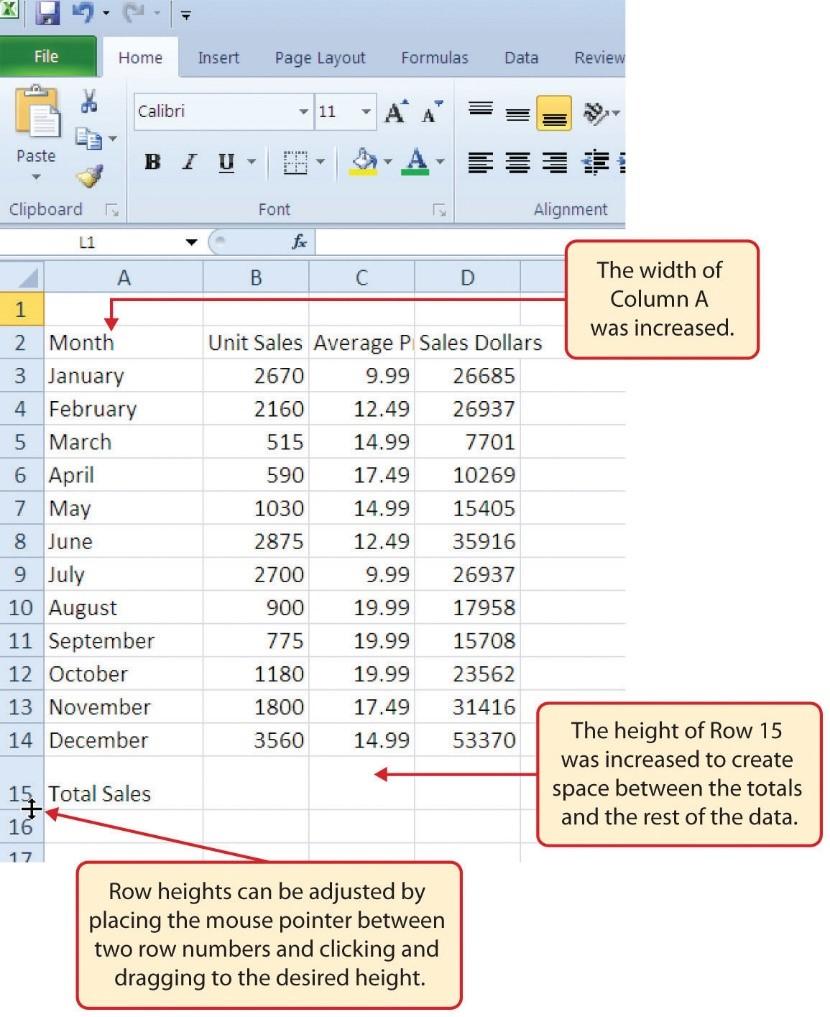
There are a few entries in the worksheet that appear cut off. For example, the last letter of the word September cannot be seen in cell A11. This is because the column is too narrow for this word. The columns and rows on an Excel worksheet can be adjusted to accommodate the data that is being entered into a cell. The following steps explain how to adjust the column widths and row heights in a worksheet:
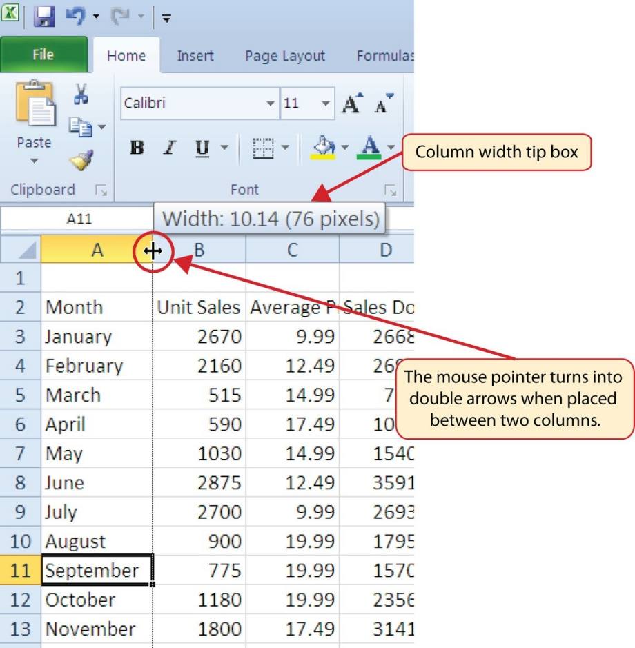
- Bring the mouse pointer between Column A and Column B in the Sheet1 worksheet, as shown in Figure 1.23. You will see the white block plus sign turn into double arrows.
- Click and drag the column to the right so the entire word September in cell A11 can be seen. As you drag the column, you will see the column width tip box. This box displays the number of characters that will fit into the column using the Calibri 11-point font which is the default setting for font/size.
- Release the left mouse button.
You may find that using the click-and-drag method is inefficient if you need to set a specific character width for one or more columns. Steps 1 through 6 illustrate a second method for adjusting column widths when using a specific number of characters:
- Click any cell location in Column A by moving the mouse pointer over a cell location and clicking the left mouse button. You can highlight cell locations in multiple columns if you are setting the same character width for more than one column.
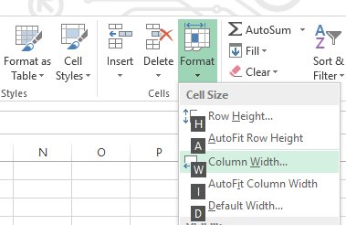
- In the Home tab of the Ribbon, left click the Format button in the Cells group.
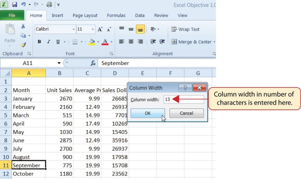
- Click the Column Width option from the drop-down menu. This will open the Column Width dialog box.
- Type the number 13 and click the OK button on the Column Width dialog box. This will set Column A to this character width (see Figure 1.24).
- Once again bring the mouse pointer between Column A and Column B so that the double arrow pointer displays and then double-click to activate AutoFit. This feature adjusts the column width based on the longest entry in the column.
- Use the Column Width dialog box (step 6 above) to reset the width to 13.
Keyboard Shortcuts
Column Width
- To set the column width, press the ALT key on your keyboard, while having that still pressed, also press the letters H, O, and W one after another. You will see options highlighted on the ribbon as you press ALT+H, then O, then W. When you press W, you will see the width dialogue box show up. Edit your desired width here.Your Excel interface when pressing H while ALT is pressed in:
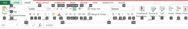 Your Excel interface when pressing O:
 Your pop-up when pressing W:
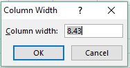
“The standard column width in Microsoft Excel 2000 is 8.43 characters; however, the actual width that you see on the screen varies, depending on the width of the font defined for the Normal style of your workbook.” More on this topic here.
Steps 1 through 4 demonstrate how to adjust row height, which is similar to adjusting column width:
- Click cell A15 by placing the mouse pointer over the cell and clicking the left mouse button.
- In the Home tab of the Ribbon, left click the Format button in the Cells group.
- Click the Row Height option from the drop-down menu. This will open the Row Height dialog box.
- Type the number 24 and click the OK button on the Row Height dialog box. This will set Row 15 to a height of 24 points. A point is equivalent to approximately 1/72 of an inch. This adjustment in row height was made to create space between the totals for this worksheet and the rest of the data.
Keyboard Shortcuts
Row Height
- Similarly to how you could set the column width above, you can use a combination of the ALT key and other keys to resize your row height. Press ALT on your keyboard, then press the letters H, O, and H one at a time. Observe how different portions of your Ribbon pop up and allow you to select them without having to move your mouse to them. This can be a great time saver!
Figure 1.25 shows the appearance of the worksheet after Column A and Row 15 are adjusted.
Skill Refresher
Adjusting Columns and Rows
- Activate at least one cell in the row or column you are adjusting.
- Click the Home tab of the Ribbon.
- Click the Format button in the Cells group.
- Click either Row Height or Column Width from the drop-down menu.
- Enter the Row Height in points or Column Width in characters in the dialog box.
- Click the OK button.
Hiding Columns and Rows
In addition to adjusting the columns and rows on a worksheet, you can also hide columns and rows. This is a useful technique for enhancing the visual appearance of a worksheet that contains data that is not necessary to display. These features will be demonstrated using the GMW Sales Data workbook. However, there is no need to have hidden columns or rows for this worksheet. The use of these skills here will be for demonstration purposes only.
- Click cell C1 in the Sheet1 worksheet by placing the mouse pointer over the cell location and clicking the left mouse button.
- Click the Format button in the Home tab of the Ribbon.
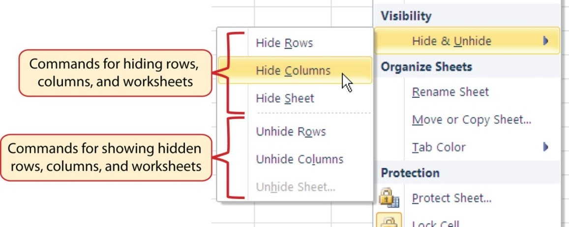
- Place the mouse pointer over the Hide & Unhide option in the drop-down menu. This will open a submenu of options.
- Click the Hide Columns option in the submenu of options (see Figure 1.26). This will hide Column C.
Keyboard Shortcuts
Hiding Columns
- Hold down the CTRL key while pressing the number 0 on your keyboard.
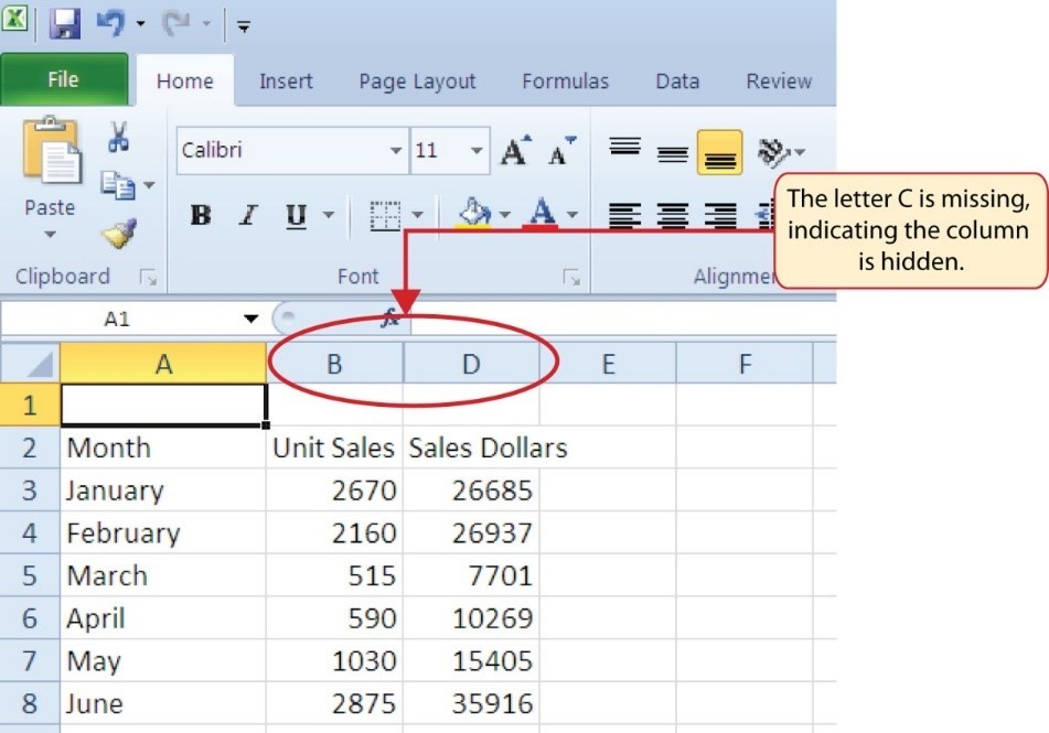
Figure 1.27 shows the workbook with Column C hidden in the Sheet1 worksheet. You can tell a column is hidden by the missing letter C.
To unhide a column, follow these steps:
- Highlight the range B1:D1 by activating cell B1 and clicking and dragging over to cell D1.
- Click the Format button in the Home tab of the Ribbon.
- Place the mouse pointer over the Hide & Unhide option in the drop-down menu.
- Click the Unhide Columns option in the submenu of options. Column C will now be visible on the worksheet.
Keyboard Shortcuts
Unhiding Columns
- Highlight cells on either side of the hidden column(s), then hold down the CTRL key and the SHIFT key while pressing the close parenthesis key ()) on your keyboard.
The following steps demonstrate how to hide rows, which is similar to hiding columns:
- Click cell A3 in the Sheet1 worksheet by placing the mouse pointer over the cell location and clicking the left mouse button.
- Click the Format button in the Home tab of the Ribbon.
- Place the mouse pointer over the Hide & Unhide option in the drop-down menu. This will open a submenu of options.
- Click the Hide Rows option in the submenu of options. This will hide Row 3.
Keyboard Shortcuts
Hiding Rows
- Hold down the CTRL key while pressing the number 9 key on your keyboard.
To unhide a row, follow these steps:
- Highlight the range A2:A4 by activating cell A2 and clicking and dragging over to cell A4.
- Click the Format button in the Home tab of the Ribbon.
- Place the mouse pointer over the Hide & Unhide option in the drop-down menu.
- Click the Unhide Rows option in the submenu of options. Row 3 will now be visible on the worksheet.
Keyboard Shortcuts
Unhiding Rows
- Highlight cells above and below the hidden row(s), then hold down the CTRL key and the SHIFT key while pressing the open parenthesis key (() on your keyboard.
Integrity Check
Hidden Rows and Columns
In most careers, it is common for professionals to use Excel workbooks that have been designed by a coworker. Before you use a workbook developed by someone else, always check for hidden rows and columns. You can quickly see whether a row or column is hidden if a row number or column letter is missing.
Skill Refresher
Hiding Columns and Rows
- Activate at least one cell in the row(s) or column(s) you are hiding.
- Click the Home tab of the Ribbon.
- Click the Format button in the Cells group.
- Place the mouse pointer over the Hide & Unhide option.
- Click either the Hide Rows or Hide Columns option.
Skill Refresher
Unhiding Columns and Rows
- Highlight the cells above and below the hidden row(s) or to the left and right of the hidden column(s).
- Click the Home tab of the Ribbon.
- Click the Format button in the Cells group.
- Place the mouse pointer over the Hide & Unhide option.
- Click either the Unhide Rows or Unhide Columns option.
Inserting Columns and Rows
Using Excel workbooks that have been created by others is a very efficient way to work because it eliminates the need to create data worksheets from scratch. However, you may find that to accomplish your goals, you need to add additional columns or rows of data. In this case, you can insert blank columns or rows into a worksheet. The following steps demonstrate how to do this:
- Click cell C1 in the Sheet1 worksheet by placing the mouse pointer over the cell location and clicking the left mouse button.
- Click the down arrow on the Insert button in the Home tab of the Ribbon (see Figure 1.28).
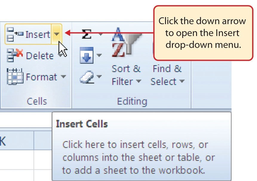
Figure 1.28 Insert Button (Down Arrow) - Click the Insert Sheet Columns option from the drop-down menu (see Figure 1.29). A blank column will be inserted to the left of Column C. The contents that were previously in Column C now appear in Column D. Note that columns are always inserted to the left of the activated cell.
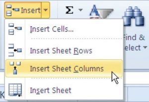
Figure 1.29 Insert Drop-Down Menu Keyboard Shortcuts
Inserting Columns
- Press the ALT key and then the letters H, I, and C one at a time. A column will be inserted to the left of the activated cell.
- Click cell A3 in the Sheet1 worksheet by placing the mouse pointer over the cell location and clicking the left mouse button.
- Click the down arrow on the Insert button in the Home tab of the Ribbon (see Figure 1.28).
- Click the Insert Sheet Rows option from the drop-down menu (see Figure 1.29). A blank row will be inserted above Row 3. The contents that were previously in Row 3 now appear in Row 4. Note that rows are always inserted above the activated cell.
Keyboard Shortcuts
Inserting Rows
- Press the ALT key and then the letters H, I, and R one at a time. A row will be inserted above the activated cell.
Skill Refresher
Inserting Columns and Rows
- Activate the cell to the right of the desired blank column or below the desired blank row.
- Click the Home tab of the Ribbon.
- Click the down arrow on the Insert button in the Cells group.
- Click either the Insert Sheet Columns or Insert Sheet Rows option.
Moving Data
Once data are entered into a worksheet, you have the ability to move it to different locations. The following steps demonstrate how to move data to different locations on a worksheet:
- Highlight the range D2:D15 by activating cell D2 and clicking and dragging down to cell D15.
- Bring the mouse pointer to the left edge of cell D2. You will see the white block plus sign change to cross arrows (see Figure 1.30). This indicates that you can left click and drag the data to a new location.
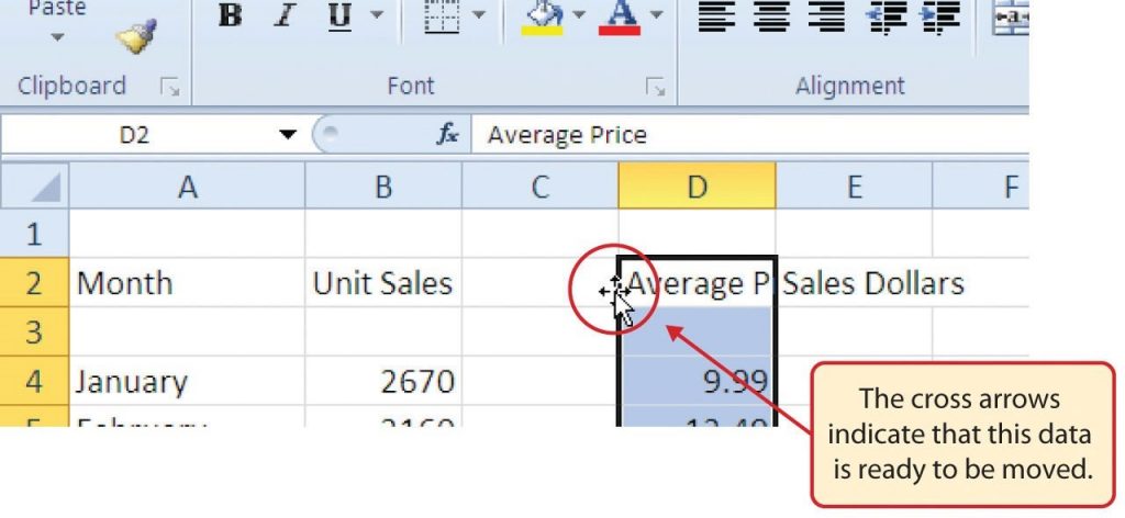
Figure 1.30 Moving Data - Left Click and drag the mouse pointer to cell C2.
- Release the left mouse button. The data now appears in Column C.
- Click the Undo button in the Quick Access Toolbar. This moves the data back to Column D.
Integrity Check
Moving Data
Before moving data on a worksheet, make sure you identify all the components that belong with the series you are moving. For example, if you are moving a column of data, make sure the column heading is included. Also, make sure all values are highlighted in the column before moving it.
Deleting Columns and Rows
You may need to delete entire columns or rows of data from a worksheet. This need may arise if you need to remove either blank columns or rows from a worksheet or columns and rows that contain data. The methods for removing cell contents were covered earlier and can be used to delete unwanted data. However, if you do not want a blank row or column in your workbook, you can delete it using the following steps:
- Click cell A3 by placing the mouse pointer over the cell location and clicking the left mouse button.
- Click the down arrow on the Delete button in the Cells group in the Home tab of the Ribbon.
- Click the Delete Sheet Rows option from the drop-down menu (see Figure 1.31). This removes Row 3 and shifts all the data (below Row 2) in the worksheet up one row.
Keyboard Shortcuts
Deleting Rows
- Press the ALT key and then the letters H, D, and R one at a time. The row with the activated cell will be deleted.
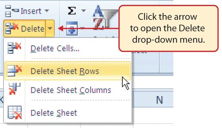
Figure 1.31 Delete Drop-Down Menu - Click cell C1 by placing the mouse pointer over the cell location and clicking the left mouse button.
- Click the down arrow on the Delete button in the Cells group in the Home tab of the Ribbon.
- Click the Delete Sheet Columns option from the drop-down menu (see Figure 1.31). This removes Column C and shifts all the data in the worksheet (to the right of Column B) over one column to the left.
- Save the changes to your workbook by clicking either the Save button on the Home ribbon; or by selecting the Save option from the File menu.
Keyboard Shortcuts
Deleting Columns
- Press the ALT key and then the letters H, D, and C one at a time. The column with the activated cell will be deleted.
Skill Refresher
Deleting Columns and Rows
- Activate any cell in the row or column that is to be deleted.
- Click the Home tab of the Ribbon.
- Click the down arrow on the Delete button in the Cells group.
- Click either the Delete Sheet Columns or the Delete Sheet Rows option.
Key Takeaways
- Column headings should be used in a worksheet and should accurately describe the data contained in each column.
- Using symbols such as dollar signs when entering numbers into a worksheet can slow down the data entry process.
- Worksheets must be carefully proofread when data has been manually entered.
- The Undo command is a valuable tool for recovering data that was deleted from a worksheet.
- When using a worksheet that was developed by someone else, look carefully for hidden columns or rows.
Attribution
Adapted by Barbara Lave from How to Use Microsoft Excel: The Careers in Practice Series, adapted by The Saylor Foundation without attribution as requested by the work’s original creator or licensee, and licensed under CC BY-NC-SA 3.0.
