
8.4 Conditional Functions
We have used functions beginning with Chapter 2 to return values based on mathematical and statistical functions like SUM, AVERAGE, and COUNT. In Chapter 3 we studied how to set up logical tests, have Excel evaluate our conditions on all items in our ranges, and then process all the values for us. In Chapter 5, we studied how to interpret directions, set up parameters and filter our data depending on a variety of criteria using Excel tables, filters, and slicers.
In this chapter, we continue our work with the College Scorecard dataset we were introduced to in Chapter 6. There, we used PivotTables and PivotCharts to summarize our dataset to gain insights into parameters that describe the cost of education and its return, enrollment trends in different types of programs, the breakdown of the student body, and more. In this chapter, we will look at alternative means of reaching the same answers by using a combination of Excel functions and formulas, we have studied in the earlier chapters.
Table 1 below provides an overview of the functions we will use to return values in Excel. Notice the pattern from SUM to SUMIF to SUMIFS, the combination of SUM + IF, or the combination of SUM + IFS, IF in the plural if you wish. The structure of these functions implies that we will SUM things up IF they meet one condition or criterion. Alternatively, we will SUM things up using the IFS ending when they must meet multiple conditions or criteria. The pattern in the composition of the functions is the same across our core mathematical and statistical functions. AVERAGE and COUNT both have so-called conditional versions that allow us to set parameters to base averaging or counting our values based upon.
| SUM | Adds values you enter in the formula. |
| SUMIF | Adds values that meet a single criterion. |
| SUMIFS | Adds all values that meet multiple criteria. |
| AVERAGE | Calculates the arithmetic mean of a range of values. |
| AVERAGEIF | Returns the average of all cells that meet a single criterion. |
| AVERAGEIFS | Returns the average of all cells that meet multiple criteria. |
| COUNT | Counts the number of cells that contain numbers. |
| COUNTIF | Counts cells using a single criterion. |
| COUNTIFS | Counts cells using multiple criteria. |
Table 1: Mathematical and Statistical Functions.
=SUMIF(range, criteria, [sum_range])
SUMIF essentially asks: what do you want to add up, based on what criteria. The SUMIF syntax starts with our function, then within the parentheses, we must tell Excel what is the range of values (text or numbers, blanks will be ignored) we want it to add up based on which criteria. Our criteria may be a single value like the number 42, or “>42″, the cell reference for where our criterion is located. If you use text or =, >, >=, etc. operators, then make sure to encase them between ” “, or Excel will return an error. The [SUM_RANGE] argument in square brackets indicates that this portion of the argument is optional, we can use it if we want to add up something other than the range we specified earlier.
For instance, we want to know how many undergraduates there are in the state of Texas. We have studied a variety of means of answering this question in previous chapters. Now, we want to use our conditional SUM function to return this value.
- Open your College Scorecard Data Excel file. (You can download a fresh copy from here.)
- Insert a few additional rows above your data table. Three or four will do.
- Considering you have over 120 columns in this data set, you can select, right-click and hide columns you do not use for the moment.
- Convert your range into an Excel table so that your formula will use your field names (column headings)
- Click into any of the cells above your the first few columns and start on your formula by typing in a = sign.
- Now, you need to specify to Excel that you want it to look at the range of State Abbreviations (STABBR), use TX as your criteria, then SUM up values in the column showing the Number of Undergraduates (UGDS). Try this on your own, or use the Figure below. Note how the Excel table structure makes it easy to see which column you are referencing, as opposed to using range references.
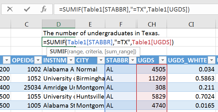
Figure 1. SUMIF Function in use. - Note the color-coded borders around each active range in the formula.
- Now, go ahead, and check the answer using other methods of getting a correct answer. This way, you can confirm that your formula has done its job. You can create an Excel table and filter it for Texas, then use the Total Row, to SUM up the Number of Undergraduates. You can also create a PivotTable using the State Abbreviation and the Number of Undergraduates fields to return an output. Do your answers match?
- Do a few more variations on this question based on cities, states, regions, types of LOCALE and more!
SUMIFS Exercise
The SUMIFS function adds all of its arguments that meet multiple criteria (support.office.com).
The syntax for SUMIFS starts with the range we want to add up, then we must specify each range with their corresponding criteria.
=SUMIFS(sum_range, criteria_range1, criteria1, [criteria_range2, criteria2], …)
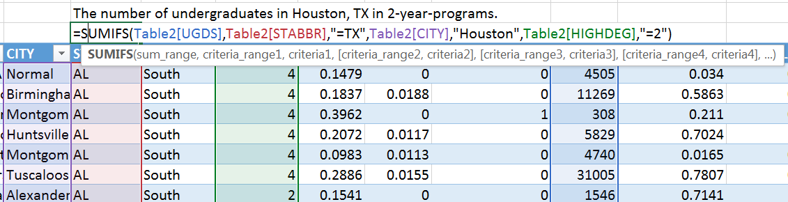
Use your College Scorecard dataset to return the number of undergraduates in the city of Houston, TX enrolled in 2- year-degree programs. Refer to your Data Dictionary to select the fields do you need to include in your calculation. List them on a sheet of paper or on a simple file on your computer you can place next to your College Scorecard data file.
If you get stuck, you can refer to this screenshot. (The table numbers [Table 1, Table 2] will reflect if you convert back to a range to pivot your data and then recreate a table…) When done, use an Excel table or a PivotTable to reach the same answer.
Consider which methods you like the most and practice those to develop not only confidence with Excel but to have multiple avenues of answering questions so that you can double-check your work.
=COUNTIF(range, criteria)
The COUNTIF syntax starts with an equal sign, followed by our function, and then within the parentheses, we must tell Excel what is the range of values we want it to count based on which criteria. As with SUMIF, our criteria may be a single value like the number 42, or “>42″, the cell reference for where our criterion is located. If you use text or =, >, >=, etc. operators, then make sure to encase them between ” “, or Excel will return an error. We do not have an optional argument as we did with SUMIF.
We want to know how many higher educational institutions there are in the state of Texas. Let’s use some of the blank cells we inserted into our sheet above our Excel table earlier to find out!
- Click into any of the cells above your the first few columns and start on your formula by typing in a = sign.
- Now, you need to specify to Excel that you want it to COUNT. Use the range of State Abbreviations (STABBR) and TX as your criteria. Try this on your own, or use the Figure below. Note how the Excel table structure makes it easy to see which column you are referencing, as opposed to using range references.
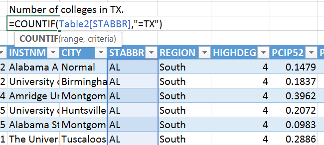
Figure 2. COUNTIF Function in use. - Note the color-coded borders around each active range in the formula.
- Once again, go ahead, and check the answer using other methods of getting a correct answer. This way, you can confirm that your formula has done its job. You can filter your Excel table for Texas, then use the Total Row, to COUNT the Institution Names or the State Abbreviations. You can also create a PivotTable using the State Abbreviation and the Institution Names fields to return an output. Do your answers match?
- Do a few more variations on this question based on cities, states, regions, types of LOCALE and more!
COUNTIFS Exercise
The COUNTIFS function applies criteria to cells across multiple ranges and counts the number of times all criteria are met (support.office.com).
=COUNTIFS(criteria_range1, criteria1, [criteria_range2, criteria2]…)
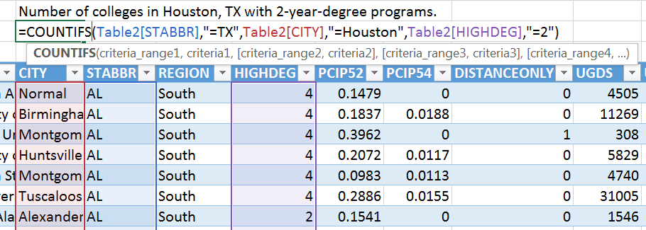
Use your College Scorecard dataset to return the number of institutions in the city of Houston, TX that offer a 2- year-degree program. Refer to your Data Dictionary to select the fields do you need to include in your calculation. List them on a sheet of paper or on a simple file on your computer you can place next to your College Scorecard data file.
If you get stuck, you can refer to this screenshot. (The table numbers [Table 1, Table 2] will reflect if you convert back to a range to pivot your data and then recreate a table…) When done, use an Excel table or a PivotTable to reach the same answer.
Again, consider which methods you like the most and practice those to develop not only confidence with Excel but to have multiple avenues of answering questions so that you can double-check your work.
More COUNTIFS Exercises:
- How many online-only education institutions are there in Arizona?
- How many academic institutions are there where more than 50% of students accept a federal loan and more than 50% accept a PELL grant in the state of California?
- How many education institutions are there in the East North Central sub-region in Large Cities?
=AVERAGEIF(range, criteria, [average_range])
The AVERAGEIF syntax will behave similarly to SUMIF. Within the parentheses, we must tell Excel what is the range of values that have our criteria, then in the optional argument in the brackets, we tell which range we want it to average if needed. For instance, we want to know what the average % of students enrolled in Business programs in Texas. Let’s use some of the remaining blank cells we inserted into our sheet above our Excel table earlier to find out!
- Click into any of the cells above your the first few columns and start on your formula by typing in a = sign.
- Now, you need to specify to Excel that you want it to AVERAGE. Use the range of State Abbreviations (STABBR) and TX as your criteria. Try this on your own, or use the Figure below. Note how the Excel table structure makes it easy to see which column you are referencing, as opposed to using range references.
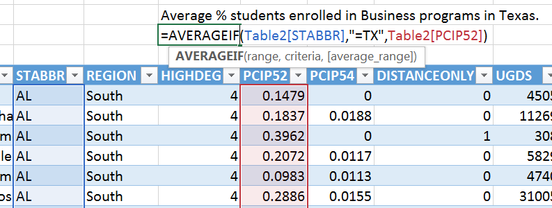
Figure 3. AVERAGEIF in use. - Note the color-coded borders around each active range in the formula.
- Once again, go ahead, and check the answer using other methods of getting a correct answer. This way, you can confirm that your formula has done its job. You can filter your Excel table for Texas, then use the Total Row, to COUNT the Institution Names or the State Abbreviations. You can also create a PivotTable using the State Abbreviation and the Institution Names fields to return an output. Do your answers match?
- Do a few more variations on this question based on cities, states, regions, types of LOCALE and more!
AVERAGEIFS Exercise
The AVERAGEIFS function returns the average (arithmetic mean) of all cells that meet multiple criteria (source: support.office.com).
=AVERAGEIFS(average_range, criteria_range1, criteria1, [criteria_range2, criteria2], …)
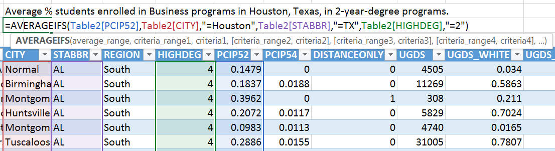
Use your College Scorecard dataset to return the average % of students enrolled in Business programs in Houston, Texas, in 2-year-degree programs. Refer to your Data Dictionary to select the fields do you need to include in your calculation. List them on a sheet of paper or on a simple file on your computer you can place next to your College Scorecard data file.
If you get stuck, you can refer to this screenshot. When done, use an Excel table or a PivotTable to reach the same answer.
More AVERAGEIFS Exercises:
- What is the average % of students enrolled in psychology in the state of California?
- What is the ACT(SAT) average in 4-year-degree institutions in the state of New York?
- What is the average percentage of students who make 25k or more 6 years after they graduate in Arizona from online-only institutions?
ATTRIBUTION
Chapter 8.3 by Emese Felvegi is licensed under CC BY 4.0
