
9.3 Creating a Budget Summary Worksheet
Linking Worksheets (Creating a Summary Worksheet)
So far we have used cell references in formulas and functions, which allow Excel to produce new outputs when the values in the cell references are changed. Cell references can also be used to display values or the outputs of formulas and functions in cell locations on other worksheets. This is how data will be displayed on the Budget Summary worksheet in the Personal Budget workbook. Outputs from the formulas and functions that were entered into the Budget Detail, Mortgage Payments, and Car Lease Payments worksheets will be displayed on the Budget Summary worksheet through the use of cell references. The following steps explain how this is accomplished:
- Click cell C3 in the Budget Summary worksheet.
- Type an equal sign =.
- Click the Budget Detail worksheet tab.
- Click cell D12 on the Budget Detail worksheet.
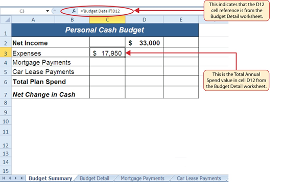
- Press the ENTER key on your keyboard. The output of the SUM function in cell D12 on the Budget Detail worksheet will be displayed in cell C3 on the Budget Summary worksheet.
Figure 9.3.1 shows how the cell reference appears in the Budget Summary worksheet. Notice that the cell reference D12 is preceded by the Budget Detail worksheet name enclosed in apostrophes followed by an exclamation point (‘Budget Detail’!) This indicates that the value displayed in the cell is referencing a cell location in the Budget Detail worksheet.
As shown in Figure 9.3.1, the Budget Summary worksheet is designed to show the expense budget for the mortgage payments and the auto lease payments. However, you will recall that we used the PMT function to calculate the monthly payments. In the Budget Summary worksheet, we need to show the total annual payments. As a result, we will create a formula that references cell locations in the Mortgage Payments and Car Lease Payments worksheets. The following steps explain how this is accomplished:
- Click cell C4 in the Budget Summary worksheet.
- Type an equal sign =.
- Click the Mortgage Payments worksheet tab.
- Click cell B5 in the Mortgage Payments worksheet.
- Type an asterisk * for multiplication.
- Type the number 12. This multiplies the monthly payments by 12 to calculate the total payments required for the year. The formula in the formula bar should read: =’Mortgage Payments’!B5*12
- Press the ENTER key on your keyboard. The value of multiplying the monthly mortgage payments by 12 is now displayed on the Budget Summary worksheet.
- Click cell C5 on the Budget Summary worksheet.
- Type an equal sign =.
- Click the Car Lease Payments worksheet tab.
- Click cell B6 in the Car Lease Payments worksheet.
- Type an asterisk * for multiplication.
- Type the number 12. This multiplies the monthly lease payments by 12 to calculate the total payments required for the year.
- Press the ENTER key on your keyboard. The value of multiplying the monthly lease payments by 12 is now displayed on the Budget Summary worksheet.
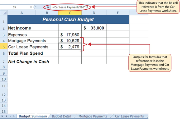
Figure 9.3.2 below shows the results of creating formulas that reference cell locations in the Mortgage Payments and Car Lease Payments worksheets.
We can now add other formulas and functions to the Budget Summary worksheet that can calculate the difference between the total spend dollars vs. the total net income in cell D2. The following steps explain how this is accomplished:
- Click cell D6 in the Budget Summary worksheet.
- Type an equal sign =.
- Type the function name SUM followed by an open parenthesis (.
- Highlight the range C3:C5.
- Type a closing parenthesis ) and press the ENTER key on your keyboard or simply press the ENTER key to close the function. The total for all annual expenses now appears on the worksheet.
- Click cell D7 on the Budget Summary worksheet. You will enter a formula to calculate Net Change in Cash in this cell.
- Type an equal sign =.
- Click cell D2.
- Type a minus sign − and then click cell D6.
- Press the ENTER key on your keyboard. This formula produces an output of $1,942, indicating our income is greater than our total expenses.
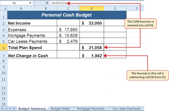
Figure 9.3.3 shows the results of the formulas that were added to the Budget Summary worksheet. The output for the formula in cell D7 shows that the net income exceeds total planned expenses by $1,942. Overall, having your income exceed your total expenses is a good thing because it allows you to save money for future spending needs or unexpected events.
We can now add a few formulas that calculate both the spending rate and the savings rate as a percentage of net income. These formulas require the use of absolute references, which we covered earlier in this chapter. The following steps explain how to add these formulas:
- Click cell E6 in the Budget Summary worksheet.
- Type an equal sign =.
- Click cell D6.
- Type a forward slash / for division and then click D2.
- Press the F4 key on your keyboard. This adds an absolute reference to cell D2.
- Press the ENTER key. The result of the formula shows that total expenses consume 94.1% of our net income.
- Click cell E6.
- Place the mouse pointer over the Auto Fill Handle.
- When the mouse pointer turns to a black plus sign, left click and drag down to cell E7. This copies and pastes the formula into cell E7.
- Save the CH2 Personal Budget file.
- Compare your work with the self-check answer key (found in the Course Files link) and then submit the CH2 Personal Budget workbook as directed by your instructor.
- Close the CH2 Personal Budget file before moving on to 2.4 – Preparing to Print.
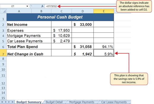
Figure 9.3.4 shows the output of the formulas calculating the spending rate and savings rate as a percentage of net income. The absolute reference shown for cell D2 prevents the cell from changing when the formula is copied from cell E6 and pasted into cell E7. The results of the formula show that our current budget allows for a savings rate of 5.9%. This is a fairly good savings rate.
Key Takeaways
- The PMT function can be used to calculate the monthly mortgage payments for a house or the monthly lease payments for a car.
- When using the PMT function, each argument must be separated by a comma.
- To calculate the monthly payment for a loan using the PMT function, the Rate and Nper arguments must be defined in terms of months. The Rate should be divided by 12 to convert it from an annual rate to a monthly rate. The Nper should be multiplied by 12 to convert the term of the loan from years to months.
- The PMT function produces a negative output if the Pv argument is not preceded by a minus sign. For the purposes of this textbook, a minus sign will be entered before the PV argument in the PMT dialog box.
Attribution
Adapted by Mary Schatz from How to Use Microsoft Excel: The Careers in Practice Series, adapted by The Saylor Foundation without attribution as requested by the work’s original creator or licensee, and licensed under CC BY-NC-SA 3.0.
