
3.4 Conditional Formatting
Learning Objectives
- Use Conditional Formatting techniques to provide flexible highlighting, applying specified formatting only when certain conditions are met. Techniques include:
- Data bars — to make it easy to visualize values in a range of cells.
- Cells Rules — to highlight values that match the requirements you specify.
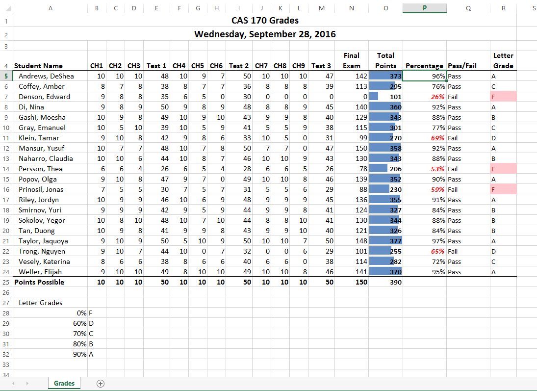
You now have all the calculations you need in your CAS 170 Grades spreadsheet. There is a lot of data here. To make it easier to pick out the most important pieces of data, Excel provides Conditional Formatting. The best thing about Conditional Formatting is that it is flexible, applying specified formatting only when certain conditions are met.
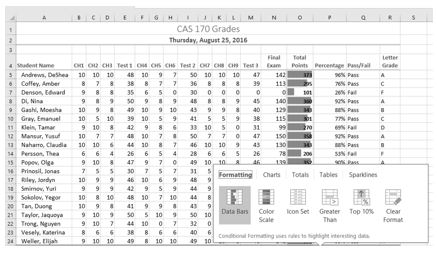
- Select the values in the Total Points column (O5:O24).
- At the bottom of your selection, click on the Quick Analysis Tool. On the Formatting tab, select Data Bars (see Figure 3.18).
Excel places blue bars on top of your values; long blue bars for larger numbers, shorter ones for smaller numbers. This makes it easier to see how well each student did in the class – without having to look at the specific numbers.
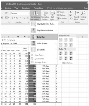
Another way to apply Data Bars is to:
- Select the range that needs data bars
- On the Home tab, in the Styles group, select Data Bars from the Conditional Formatting tool.
- From there you can select data bars of different colors and opacities (see Figure 3.19).
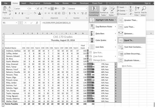
- Select the Letter Grades (R5:R24).
- On the Home tab, in the Styles group, select Highlight Cell Rules from the Conditional Formatting tool (see Figure 3.20).
- Select Equal To
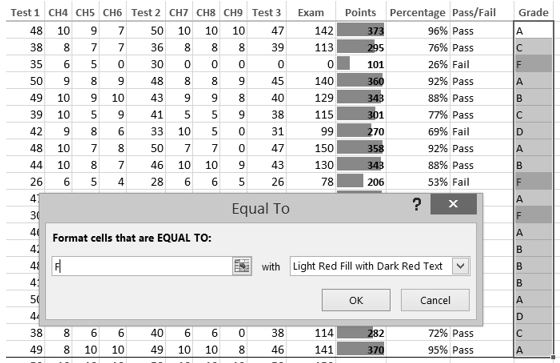
- Fill out the Equal to dialog box so that cells that are equal to: F have Light Red Fill with Dark Red Text (see Figure 3.21).
Let’s try that one more time – to highlight those students who are passing the class. This time we will use the Pass/Fail text in the Pass/Fail column. If the text for a student is Pass we want the cell to be formatted with a yellow fill with dark yellow text.
- Select the Pass/Fail grades (Q5:Q24).
- On the Home tab, in the Styles group, select Highlight Cell Rules from the Conditional Formatting tool (see Figure 3.20).
- Select Equal To
- Fill out the Equal to dialog box so that cells that are equal to: Pass have Yellow Fill with Dark Yellow Text. (To find the Yellow Fill with Dark Yellow text option, click the the down arrow at the end of the last (with) box).
You do not have to use the default styles to make your data stand out. You can set any formatting you want. When you do, it is probably a good idea to include other styling in addition to color. Your spreadsheet might be printed in black and white. You would hate to lose your Conditional formatting. Now we are going to use conditional formatting to display any Percentages that are less than 60% with red text formatted in bold and italic.
- Select the Percentage grades (P5:P24).
- On the Home tab, in the Styles group, select Highlight Cell Rules from the Conditional Formatting tool (see Figure 3.20).
- Select Less Than
- Fill out the Less Than dialog box so that cells that are less than .6 will be have conditional formatting. But, instead of using the default red text on a light red fill, press the down arrow at the end of that box and select Custom Format.
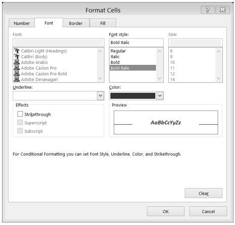
- On the Font tab of the Format Cells dialog box, in the Font style box, select Bold Italic. In the Color box, select Red (see Figure 3.22).
- Press OK. Then press OK again.
Conditional Formatting is valuable in that it reflects the current data. It changes to reflect changes in the data. To test this, delete DeShea’s final exam score. (Select N5. Press Delete on your keyboard.) Suddenly, DeShae is failing the course and the Conditional Formatting reflects that. This is a little unfair to DeShae – who has worked so hard this quarter. Let’s give him back his grade. Press CTRL Z (Undo). His test score reappears and the Conditional formatting reflects that as well.
Making Changes
What if you have made a mistake with your Conditional Formatting? Or, you want to delete it altogether? You can use the Conditional Formatting Manage Rules tool. In our example, we want to remove the conditional formatting rule that formats the Pass text with yellow. We are also going to modify the minimum passing percentage for the conditional formatting rule that is applied to the percentages.
- On the Home Tab, in the Styles Group, select Manage Rules at the very bottom of the Conditional Formatting drop-down list.
- Show formatting rules for: This Worksheet (see Figure 3.23).
- We don’t really need to highlight the students who are passing the class, so select that rule in the Rules Manager and press the Delete Rule button.
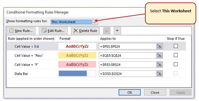
Figure 3.23 Conditional Formatting Manage Rules In a previous exercise (the IF function), we decided that students were failing if they got a percentage score of less than 70%, so the Conditional Formatting rule in the Percentage column needs repair.
- Select the rule that reads Cell Value <0.6.
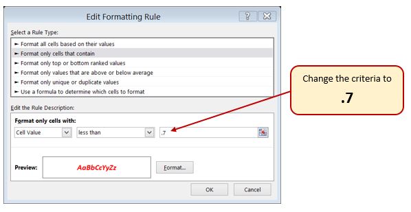
- Select the Edit Rule button, and change the .6 to .7 (see Figure 3.24).
- Click OK (or Apply) twice. Double check that your completed workbook matches Figure 3.25.
Setting the Print Area
Before you consider this workbook finished, you need to prepare it for printing. The first thing you will do is set the Print Area so that the table of Letter Grades in A27:B32 does not print.
- Select A1:R25. This is the only part of the worksheet that you want to have print.
- On the Page Layout ribbon, click the Print Area button. Choose Set Print Area from the menu.
Next you will preview the worksheet in Print Preview to check that the print area setting worked, as well as make sure it is printing on one page.
- View the workbook in Print Preview.
- Set the page orientation to Landscape.
- Change the page scaling if needed so that the entire worksheet prints on one page.
- Save and close the CH3 Gradebook workbook.
- Compare your work with the self-check answer key (found in the Course Files link) and then submit the CH3 Gradebook workbook as directed by your instructor.
Attribution
3.3 Conditional Formatting by Noreen Brown and Mary Schatz, PCC.EDU, is licensed under CC BY 4.0
