
6.5 Fashion Data Practice
Excel Chapter 6 – Practice 1
Top 200 Fashion Data
Written guide to accompany: https://youtu.be/W6NM9X5GMBQ
We are going to practice PivotTables with the data set from last week. Last week, we did an ExcelTable. This week we are going to do a PivotTable just to see how much more flexible a PivotTable is than an ExcelTable and how we can do things differently with it.
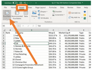
Open the Top 200 Fashion Companies Data.xlsx file.
Click anywhere into the table on the left, go to the Insert Tab, click the PivotTable icon.
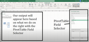
Confirm the range (trust Excel, don’t edit it), and then in a new sheet I’m going to get a blank canvas on the left, and on the right, I’m going to have the PivotTable field selector.
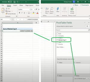
If I click on the Market Cap # field name on the right-hand side, Excel is going to recognize that I’m dealing with numbers here and put that number under the Values field and show me what the SUM of the Market Cap # is for ALL of the companies in the Top 200. This is a SUPER QUICK way for me to get a Grand Total!
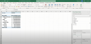
Next, I’m going to click on the Country field name and see where Excel automatically sorts it.
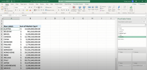
What I get is really great summary data already! I didn’t have a large data set, but I did have just enough that it was impossible for me to see it on one page. Now I have the summaries by country and I can do things with the SUM of Market Cap #, like sort it from largest to smallest or filter out values I don’t want to see. Try some of them!
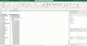
From last week I already knew that the U.S. had the highest combined market cap and France, and Spain was in the top three alongside it, but what I had to do in an Excel Table to figure this out was to filter or use a slicer and then arrange values or Subtotals accordingly.
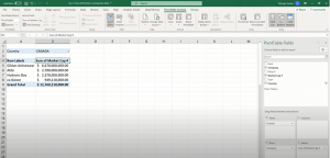
Here, what I can do is flexibly move things around!
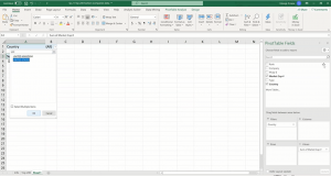
If I want to see the Market Cap # for the United States and I want to see the companies, I can quickly Pivot my data that I can sort and filter. I can have that PivotTable field selector display the country, the company, and the SUM of the Market Cap # in a flexible manner.
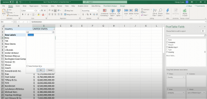
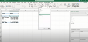
Do I want to change it to Canada to do that comparison?
I can go ahead and do that quickly and effectively by changing the filter.
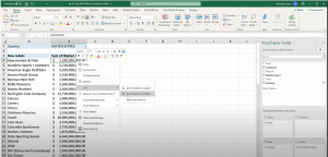
Do I want to include the type of company that exists?
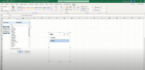
It might actually be better for me to put the type under the filter, or I can remove the type and I can put it in a slicer for type.
I can quickly and effectively change the country and then the company type and the total will update for me at the end of that pivot table.
So, what I want you to do is play with this for a few minutes and then pull up that quiz and answer the questions you get using a PivotTable.
This week, you’ll have 15 questions, so please go ahead and practice before starting your attempt. Do your best and if you run into issues, please seek help from a tutor or come see me during office hours.
Good luck, have fun, go Excel!
