
3.1 More Ways to Use Formulas and Functions
Learning Objectives
- Review the use of the =MIN, MAX, AVERAGE functions.
- Examine the Quick Analysis Tool to create standard calculations, formatting, and charts very quickly.
- Create Percentage calculation.
– Use the Smart Lookup tool to acquire additional information about percentage calculations.
– Review the use of Absolute cell reference in a division formula.
Another use for =MAX
Before we move on to the more interesting calculations we will be discussing in this chapter, we need to determine how many points it is possible for each student to earn for each of the assignments. This information will go into Row 25. The =MAX function is our tool of choice.
Download Data File: Ch-3-Data_File
- Open the data file CH3 Data File and save the file to your computer as CH3 Data [Your Name]. Go to the Grades sheet, which is the second sheet from the left at the bottom of your Excel interface.
- Make B25 your active cell.
- Start typing =MAX (See Figure 3.2) Note the explanation you see on the offered list of functions. You can either keep typing ( or double click MAX from the list.

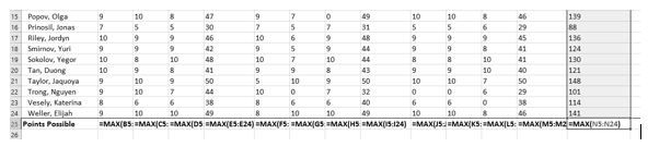
Figure 3.2 Entering a function - Select the range of numbers above row 25. Your calculation will be: =MAX(B5:B24)
- Now, use the Fill Handle to copy the calculation from Column B through Column N.
Note that as you copy the calculation from one column to the next, the cell references change. The calculation in column B reads: =MAX(B5:B24). The one in column N reads: =MAX(N5:N24). These cell references are relative references.
By default, the calculations that Excel copies change their cell references relative to the row or column you copy them to. That makes sense. You wouldn’t want column N to display an answer that uses the values in column L.
Want to see all the calculations you have just created? Press Ctrl ~ (See Figure 3.3.) Ctrl ~ displays your calculations (formulas). Pressing Ctrl ~ a second time will display your calculations in the default view – as values.
PRACTICE
Insert a row below the points possible and calculate lowest possible and average values for each assignment and exam.
Quick Analysis Tool
The Quick Analysis Tool allows you to create standard calculations, formatting, and charts very quickly. In this exercise we will use it to insert the Total Points for each student in Column O.
Be sure to press Ctrl ~ to return your spreadsheet to the normal view (the formula results should display, not the formulas themselves).
- Select the range of cells B5:N25
- In the lower right corner of your selection, you will see the Quick Analysis tool (see Figure 3.4).
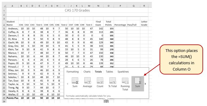
Figure 3.4 Quick Analysis Tool - When you click on it, you will see that there are a number of different options. This time we will be using the Totals option. In future exercises, we will use other options.
- Select Totals, and then the SUM option that highlights the right column (see Figure 3.5). Selecting that SUM option places =SUM() calculations in column O.
Percentage calculation
Column P requires a Percentage calculation. Before we launch in to creating a calculation for this, it might be handy to know precisely what it is we are looking for. If you are connected to the internet, and are using Excel 2016, you can use the Smart Lookup tool to get some more information.
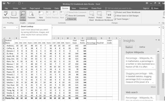
- Select cell P4.
- Find the Smart Lookup tool on the Review tab (see Figure 3.6).
- Press the Smart Lookup tool to find more about Percentage calculations.
If this is the first time you have used the Smart Lookup tool, you may need to respond to a statement about your privacy. Press the Got it button.
I think the first Wikipedia article does a pretty good job explaining the calculation, don’t you?
Now that we know what is needed for the Percentage calculation, we can have Excel do the calculation for us. We need to divide the Total Points for each student by the Total Points of all the Points Possible. Notice that there is a different number on each row – for each student. But, there is only one Total Points Possible – the value that is in cell O25.
- Make sure that P5 is your active cell.
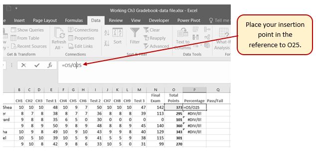
- Press = then select cell O5. Press /, then cell O25. Your calculation should look like this: =O5/O25. The result of the formula should be 0.95641026. (So far, so good. DeShea Andrews is doing well in this class – with a percentage grade of almost 96%. Definitely an “A”!)
- Next use the Fill handle to copy the calculation down through row 24 to calculate the other students’ grades. You should get the error message #DIV/0!. This error message reminds us that you can’t divide a number by 0 (zero). And that is just what is happening. If you look at the calculation in P9, the calculation reads: =O9/O29. The first cell reference is correct – it points to Moesha Gashi’s total points for the class. But the second reference is wrong. It points to an empty cell – O29.
Before copying the calculation, we have to make the second reference (O25) an absolute cell reference. That way, when we copy the formula down, the cell reference for O25 will be locked and will not change.
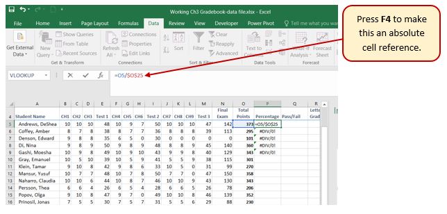
- Make P5 your active cell. In the Formula Bar click on O25 (see Figure 3.7).
- Press F4 (on the function keys at the top of your keyboard). That will make the O25 reference absolute. It will not change when you copy the calculation (see Figure 3.8). (If you are working on a laptop and do not have an F4 function key, you can type in a $ before the O and another one before the 25.)
- The calculation now looks like this: =O5/$O$25.
- Use the Fill Handle to copy the formula down through P24 again. Now, when you copy the formula, you will get correct values for all of the students.
Those long decimals are a bit nonstandard. Let’s change them to % by applying cell formatting.
- Select the range P5:P24.
- On the Home tab, in the Number Group, select the % (Percent Style) button.
Skill Refresher
Absolute References
- Click in front of the column letter of a cell reference in a formula or function that you do not want altered when the formula or function is pasted into a new cell location.
- Press the F4 key or type a dollar sign ($) in front of the column letter and row number of the cell reference.
Key Takeaways
- Functions can be created using cell ranges or selected cell locations separated by commas. Make sure you use a cell range (two cell locations separated by a colon) when applying a statistical function to a contiguous range of cells.
- To prevent Excel from changing the cell references in a formula or function when they are pasted to a new cell location, you must use an absolute reference. You can do this by placing a dollar sign ($) in front of the column letter and row number of a cell reference or by using the F4 function key.
- The #DIV/0 error appears if you create a formula that attempts to divide a constant or the value in a cell reference by zero.
Attribution
3.1 More on Formulas and Functions by Noreen Brown and Mary Schatz, PCC.EDU, is licensed under CC BY 4.0
